Thin Lens Equation Interactive Calculator

Getting the position of a lens right—whether you're setting up a camera, microscope, or a machine vision system—comes down to understanding how object distance, image distance, and focal length all work together. With the Thin Lens Equation Interactive Calculator, you enter any two of these values to solve for the missing one or calculate related values like magnification and lens power. These basic relationships are used constantly in cameras, telescopes, eyeglasses, robotic positioning, and inspection systems. Below you'll find the main formulas, a detailed engineering example, some background theory, and a solid FAQ for troubleshooting or clarification.

What is the thin lens equation?

The thin lens equation is a basic formula linking object distance, image distance, and lens focal length. If you know any two, you can directly solve for the third. This is one of the first tools you'll reach for in practical optics work.

Simple Explanation

If you've ever used a magnifying glass to focus sunlight to a sharp spot, that spot is the focal point. The thin lens equation lets you figure out exactly where that sharp image appears based on your object position and lens focal length. The relationships are simple: as the object gets closer, the image moves farther away, and vice versa—the equation does the bookkeeping.

📐 Browse all 1000+ Interactive Calculators

How to Use This Calculator

1. Pick what you want to solve for using the dropdown—image distance, object distance, focal length, magnification, lens power, or do a complete parameter check.
2. Type your known values into the visible fields (all in millimeters unless otherwise noted). Depending on what you're solving for, enter object distance, image distance, focal length, and/or object height.
3. If you just want to test how it works, hit Try Example to auto-fill typical values for the selected mode.
4. Click Calculate to get the result.

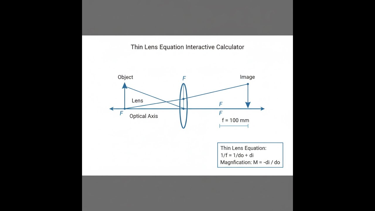
Ray Diagram

Interactive Calculator

<> Embed this calculator → <> Embed this animation calculator →

Governing Equations

If you know any two of object distance, image distance, or focal length, these equations will let you calculate the third. Plug in your values and check your units.

Use these for calculating magnification and image height.

Lens power is mainly for vision correction and some optical setups—here’s the formula in diopters.

Newtonian form is sometimes more convenient if you’re measuring distances from focal points, not from the lens center:

Simple Example

Object distance (d_o): 200 mm
Focal length (f): 100 mm
Solving for image distance: 1/d_i = 1/100 − 1/200 = 0.005, so d_i = 200 mm
Magnification: M = −200/200 = −1.0x (real, inverted, same size as object)

Theory & Practical Applications

Geometric Optics Foundation

The thin lens equation is a workhorse in geometric optics; it applies when lens thickness is much less than the radius of curvature, and rays enter at small angles—think within about 10 degrees of the optical axis. This keeps math linear and manageable. Real lenses don’t behave perfectly: you’ll run into aberrations like spherical aberration, coma, and astigmatism, especially if you push for wide fields or demanding resolution. In high-precision optics (microscopy, lithography), those effects are minimized with complex multi-lens designs and careful surface shaping. But for quick design or initial sizing, the thin lens equation gets you most of the way.

Getting sign conventions right is non-negotiable if you want correct results. Typically, positive distances are measured in the direction light travels. With a converging (convex) lens and a real object, you’ll get a real, inverted image if the object is outside the focal length. Move the object inside the focal length, and you get a virtual, upright, magnified image—that’s how magnifiers work. A diverging (concave) lens always produces a virtual, upright, reduced image from a real object. That’s why these are used in glasses for nearsightedness and also for some laser beam expanders.

Critical Distance Relationships

Certain object-image setups are important in day-to-day design. Put your object exactly at twice the focal length (d_o = 2f), and the image will appear the same distance on the other side (d_i = 2f), same size as the object but inverted—handy in relay optics. As the object gets closer to the focal point, the image distance heads toward infinity. This is what collimators use to produce parallel beams. If d_o equals f, the equation gives an infinite image distance, so rays leave parallel and you don’t get a focused image.

When setting up a camera or inspection system, the thin lens formula isn’t just a curiosity—it tells you exactly where to put the sensor and how things change if your object moves. For example, if you have a 25mm lens focusing on a circuit board 100mm away, you’ll get the image at 33.33mm behind the lens and a magnification of about -0.333x. Change the object distance, and you must move the sensor to keep focus. Even a few millimeters of movement demands tight mechanical tolerances, especially if you want sharp images or high-resolution inspection.

Power and Diopters in Optical Design

Diopters (inverse meters) are useful if you need to add up optical powers—as in eyeglass prescriptions or some optical systems with stacked thin lenses. Add lens powers directly if they’re very close together. The math breaks down for lenses farther apart, or for thick lenses, and then you need to use the principal plane method or dive into matrix analysis. Telephoto camera lenses use this trick to shrink long focal lengths into smaller physical assemblies by carefully combining positive and negative lenses.

The thin lens rule is only reliable while lens thickness is small relative to diameter or focal length. If the lens is thick (over 10% of diameter or 5% of focal length), the actual imaging location shifts. In this case, you need principal plane calculations or ray-tracing tools to get usable numbers—especially in multi-element assemblies. For very precise optical systems or thick glass, basic lens formulas are not enough.

Real-World Engineering Applications

Small camera modules, like those in phones, push thin lens equations to their limits. A phone camera lens of 4.5mm focal length typically sits about 5.8mm from the sensor. For distant objects, you set the image plane to match the focal length, but to focus on something closer (say 250mm away), you need to increase lens-to-sensor distance by under 0.1mm. That’s why autofocus actuators in phones only require tiny travel, but they must move quickly and precisely.

In laser machining, you use the lens equation with beam propagation formulas to estimate spot size and depth of focus. The focal length, working distance, and aperture size all trade off: you design the lens setup depending on the workpiece and the required focus range. The numbers are not always pretty—going for a small spot increases beam divergence and tightens tolerances on everything from lens position to flatness.

Projectors have to throw a tiny image onto a big screen, so you’ll use the thin lens calculation to pick the throw ratio, focal length, and make sure the image fills the display. Variable zoom and lens shift add complexity, but at the core, it’s still the same old formula. Don’t forget about chromatic aberration: unless you use special glass or extra lens elements, you’ll get colored fringes at high contrast edges.

Worked Example: Industrial Machine Vision System Design

Suppose you’re designing a system to inspect automotive bearing races, which are 18mm across, and you need to resolve features at the 3.2 micron/pixel level. You’re constrained to a 300mm working distance due to mechanical clearance. Here’s how you’d work through the numbers for focal length, sensor size, and depth of field using f/5.6:

Step 1: Determine Required Magnification

Sensor pixel pitch is 3.2 μm. For a 20mm field (with some margin), you need 6250 pixels across. Using a common 2/3" sensor (8.8mm wide, 2752 pixels, 3.2μm pixel), actual magnification will be about 0.44x (8.8mm/20mm).

Step 2: Calculate Image Distance

From magnification: 0.44 = -d_i / 300
So d_i = -132mm (the sign and side matter; usually you take the absolute value for sensor placement).

Step 3: Calculate Focal Length

1/f = 1/300 + 1/132, so f ≈ 91.7mm. You’d likely select a standard 90mm lens as the closest available.

Step 4: Verify Actual Performance with Standard Lens

Plug back into the formula to check. With a 90mm lens at 300mm object distance, image forms 128.6mm away. Magnification is -0.429x, so your field of view covers the part fine.

Step 5: Calculate Depth of Field

With f/5.6 and a circle of confusion twice the pixel size (6.4μm), the DOF comes out to about 4.3mm. That covers typical part thickness tolerance. If you need more, you can stop down to f/8, trading off light and exposure.

This is a typical approach for real-world vision system sizing—choose your constraints, run through the math, and check your chosen lens and camera will do the job.

Edge Cases and Failure Modes

The thin lens equation doesn't cover everything. Whenever d_o equals f, the math gives an infinite image distance—parallel light, no real image focus. This crops up in collimators or alignment setups. Calculating too close to this condition can lead to unstable or meaningless results if you’re not careful with your math or programming. For diverging lenses and virtual images, sign conventions can trip you up—keep track of which side your image is on, and always double-check signs before you order hardware or cut metal.

Chromatic aberration is another practical limitation. Glass lenses focus different colors at slightly different distances—this shows up as edge fringing when using broad-spectrum light. You can partly fix this with doublet/triplet lenses or by using monochromatic sources, but if you need true achromatism, expect a much more expensive and complex optical train. For more on related engineering design, check out the full calculator library here.

Frequently Asked Questions

Video Walkthrough - How to Use This Calculator