Signal To Noise Ratio Interactive Calculator

Designing a reliable signal chain means knowing exactly how much your useful signal stands above the noise floor — whether you're troubleshooting a sensor input, speccing a wireless link, or validating an audio stage. Use this Signal-to-Noise Ratio calculator to calculate SNR in decibels, linear power ratio, or work backwards from a known SNR to find required signal or noise power levels. It matters across telecommunications, precision instrumentation, audio engineering, and motion control systems where sensor noise directly affects positioning accuracy. This page includes the core SNR formulas, a worked satellite downlink example, noise source theory, and a full FAQ.

What is Signal-to-Noise Ratio?

Signal-to-Noise Ratio (SNR) is a measure of how strong your desired signal is compared to the background noise in a system. A higher SNR means a cleaner, more reliable signal — a lower SNR means noise is drowning out your information.

Simple Explanation

Think of it like trying to hear someone talk at a party. If they're speaking loudly in a quiet room, that's high SNR — their voice stands out clearly. If there's a loud crowd and they're whispering, that's low SNR — the noise is overwhelming the signal you care about. In electronics and communications, SNR tells you exactly how much "room" your signal has above the noise floor, expressed as a ratio in decibels (dB).

📐 Browse all 1000+ Interactive Calculators

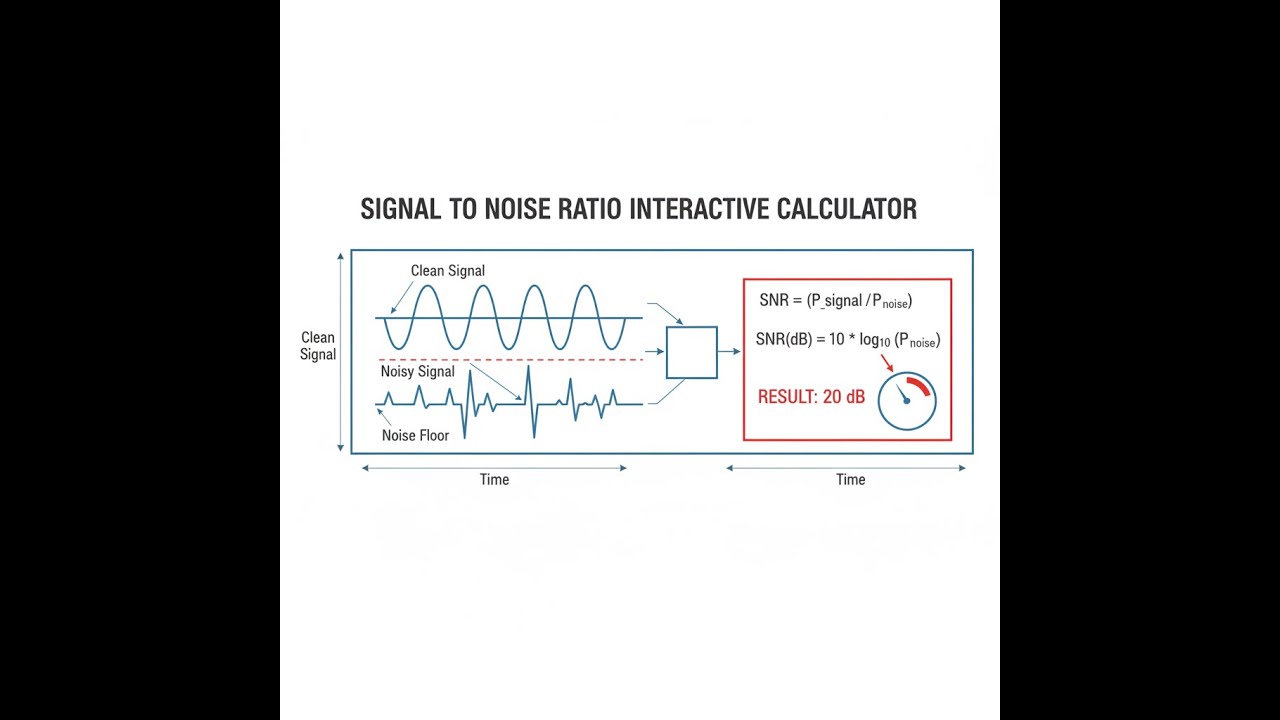
Signal and Noise Diagram

How to Use This Calculator

1. Select your Calculation Mode from the dropdown — choose from power ratio, voltage ratio, dB conversion, or reverse calculations.
2. Enter the required input values for your selected mode (signal power in W, noise power in W, voltage in V, SNR in dB, or linear ratio).
3. Review the input fields — all values must be positive numbers; voltage and power inputs cannot be zero or negative.
4. Click Calculate to see your result.

Interactive SNR Calculator

SNR Equations and Definitions

Use the formula below to calculate SNR from a power ratio.

Use the formula below to calculate SNR from a voltage ratio.

Use the formula below to calculate the linear power ratio from SNR in dB.

Use the formula below to calculate noise power when signal power and SNR are known.

Where:

• SNR_dB = Signal-to-Noise Ratio in decibels (dB)
• P_signal = Signal power in watts (W)
• P_noise = Noise power in watts (W)
• V_signal = Signal voltage RMS in volts (V)
• V_noise = Noise voltage RMS in volts (V)
• log₁₀ = Logarithm base 10

Simple Example

Signal power = 100 W, Noise power = 1 W.
Linear ratio = 100 / 1 = 100.
SNR = 10 × log₁₀(100) = 10 × 2 = 20 dB.
Result: Good signal quality — suitable for most applications.

Theory & Practical Applications of Signal-to-Noise Ratio

Fundamental Physics of Signal-to-Noise Ratio

Signal-to-Noise Ratio quantifies the relative strength of a desired signal compared to background noise in any transmission or measurement system. The logarithmic decibel scale provides an intuitive framework because human perception of signal quality is roughly logarithmic, and practical SNR values in engineering span many orders of magnitude. A 3 dB improvement represents a doubling of signal power relative to noise, while 10 dB represents a tenfold increase. The decibel formulation compresses this wide dynamic range into manageable numbers.

The distinction between the 10× and 20× multipliers in SNR calculations reflects fundamental power relationships. Power is proportional to the square of voltage or current in resistive systems. When calculating SNR from voltage measurements, we use 20×log₁₀ because the power ratio equals the voltage ratio squared: 10×log₁₀(V²ₛ/V²ₙ) = 20×log₁₀(Vₛ/Vₙ). This mathematical equivalence holds only when signal and noise experience identical impedance conditions—a critical assumption that fails in some RF matching networks and non-linear systems.

Noise Sources and Their Physical Origins

Thermal noise (Johnson-Nyquist noise) arises from random electron motion in conductors at temperatures above absolute zero. This fundamental noise source has a power spectral density of Pₙ = 4kTBR, where k is Boltzmann's constant (1.38×10⁻²³ J/K), T is absolute temperature, B is bandwidth, and R is resistance. At room temperature (290 K) in a 50Ω system with 1 MHz bandwidth, thermal noise power equals approximately -114 dBm. This sets a fundamental floor for SNR in any practical system.

Shot noise originates from the discrete nature of charge carriers crossing potential barriers in semiconductor junctions and vacuum tubes. Its power spectral density follows Pₙ = 2qIB, where q is electron charge and I is DC current. In photodetectors operating at low light levels, shot noise dominates thermal noise and establishes the quantum limit of optical detection. A photodiode with 1 μA photocurrent in 1 MHz bandwidth generates shot noise current of approximately 0.57 pA/√Hz.

Flicker noise (1/f noise) exhibits power spectral density inversely proportional to frequency and dominates at low frequencies in most active devices. Its physical origin relates to surface traps and defects in semiconductors. Precision instrumentation operating below 10 Hz must account for 1/f noise through chopping techniques or AC coupling strategies. The 1/f corner frequency—where flicker noise equals white noise—ranges from 1 Hz in precision op-amps to 1 MHz in poorly fabricated transistors.

SNR Requirements Across Engineering Disciplines

Digital communication systems require SNR values determined by modulation scheme and acceptable bit error rates. Binary Phase Shift Keying (BPSK) achieves a bit error rate of 10⁻⁶ with approximately 10.5 dB SNR, while 64-QAM demands roughly 24 dB for equivalent performance. These thresholds emerge from the statistical overlap between signal constellation points in the presence of Gaussian noise. Modern coding techniques like turbo codes and LDPC shift these requirements toward the Shannon limit, extracting reliable information from channels with SNR below 0 dB.

Audio applications exhibit human-perceptible quality thresholds. Professional recording studios target SNR exceeding 90 dB (16-bit) or 120 dB (20-bit) to preserve dynamic range across the full audible spectrum. Consumer FM radio operates acceptably at 40-50 dB SNR, while AM radio remains intelligible down to 20 dB. These differences reflect both the information content of speech versus music and the psychoacoustic masking effects where loud signals obscure nearby noise.

Instrumentation and measurement systems face SNR limitations from the fundamental physics of sensors and amplifiers. A precision 24-bit ADC theoretically provides 144 dB dynamic range, but achieving this requires input SNR exceeding 140 dB—a formidable challenge when thermal noise at room temperature in a 1 kHz bandwidth already sits at -124 dBm in 50Ω. Practical high-resolution measurement systems employ synchronous detection (lock-in amplification), where signal bandwidth is collapsed to millihertz levels, dramatically improving SNR through the reduction of integrated noise power.

Non-Obvious Engineering Considerations

The bandwidth-SNR tradeoff represents a fundamental design constraint often overlooked in preliminary system analysis. Doubling bandwidth doubles the integrated noise power, reducing SNR by 3 dB if signal power remains constant. This relationship drives the prevalence of narrowband systems in weak-signal applications like deep-space communications and radio astronomy. The 305-meter Arecibo telescope (when operational) achieved extraordinary sensitivity partly by processing bandwidths as narrow as 1 Hz, enabling detection of signals billions of times weaker than background noise when integrated over time.

Coherent and non-coherent detection strategies produce vastly different SNR requirements for equivalent error performance. A coherent receiver maintaining phase-locked local oscillators extracts maximum information from received signals, while envelope detectors sacrifice 3-4 dB in required SNR. This difference appears modest but becomes critical in power-constrained systems like satellite communications, where a 3 dB improvement halves required transmit power—potentially saving millions in launch costs and solar panel mass.

Pre-emphasis and de-emphasis filtering exploits the non-uniform spectral distribution of noise and signal energy. FM broadcasting applies 75 μs pre-emphasis to boost high-frequency signal content before transmission, then applies complementary de-emphasis at the receiver. Because most noise enters during transmission and receiver front-end stages, this technique improves subjective SNR by 10-15 dB for speech and music, where information concentrates at mid-frequencies. The strategy fails for wideband data where spectral shaping violates signal integrity requirements.

Worked Example: Satellite Downlink Analysis

Consider a satellite communication downlink operating at 11.7 GHz with the following realistic parameters:

• Satellite transmit power: 50 W (47 dBW)
• Transmit antenna gain: 34 dBi
• Distance to ground station: 38,500 km (geostationary orbit)
• Receive antenna gain: 42 dBi (1.8 m dish)
• System noise temperature: 85 K (low-noise amplifier cooled to cryogenic temperature)
• Required bandwidth: 36 MHz (single transponder)

Step 1: Calculate Free-Space Path Loss

The path loss at 11.7 GHz over 38,500 km follows:

L_path = 20×log₁₀(4πd/λ) where λ = c/f = 3×10⁸/(11.7×10⁹) = 0.02564 m

L_path = 20×log₁₀(4π × 3.85×10⁷ / 0.02564) = 20×log₁₀(1.887×10¹⁰) = 205.5 dB

Step 2: Calculate Received Signal Power

P_received = P_transmit + G_tx + G_rx - L_path

P_received = 47 dBW + 34 dBi + 42 dBi - 205.5 dB = -82.5 dBW = -52.5 dBm

Step 3: Calculate Noise Power

Thermal noise power follows P_noise = kTB

P_noise = (1.38×10⁻²³ J/K) × (85 K) × (36×10⁶ Hz) = 4.22×10⁻¹⁴ W

P_noise = 10×log₁₀(4.22×10⁻¹⁴ / 10⁻³) = -133.7 dBm

Step 4: Calculate SNR

SNR = P_signal - P_noise = -52.5 dBm - (-133.7 dBm) = 81.2 dB

This exceptional SNR of 81.2 dB enables high-order modulation schemes like 32-APSK used in modern satellite broadcasting, delivering data rates exceeding 100 Mbps per transponder. The cryogenic cooling of the LNA contributes approximately 12 dB compared to room-temperature operation, demonstrating why ground stations invest in complex refrigeration systems.

Without cooling, the system noise temperature would rise to approximately 300 K, degrading SNR to 75.7 dB—still excellent but limiting modulation options and requiring more robust error correction with corresponding throughput penalties.

Step 5: Link Margin Analysis

For 32-APSK with rate-3/4 FEC, required SNR is approximately 16 dB for 10⁻⁷ BER. The actual link margin becomes:

Margin = 81.2 dB - 16 dB = 65.2 dB

This substantial margin accounts for rain fade (up to 8 dB at 11.7 GHz in severe storms), antenna pointing errors (2-3 dB), atmospheric absorption variations (1-2 dB), and equipment aging (3-4 dB). The remaining 45+ dB provides service availability exceeding 99.9% under all but the most extreme weather conditions. Engineers could alternatively reduce transmit power or antenna size to achieve target availability with lower cost, or improve to 64-APSK for higher throughput by consuming 6 dB of the margin while maintaining reliability.

Applications in Control Systems and Robotics

For the engineering calculator library at FIRGELLI's calculator collection, SNR analysis directly impacts sensor selection and signal conditioning in motion control applications. Position encoders in linear actuator systems must deliver sufficient SNR to resolve target position increments without false counts from electrical noise. A 0.01 mm positioning accuracy requirement with quadrature encoding demands SNR exceeding 20 dB when encoder pulse edges must be distinguished from switching noise in adjacent motor drives.

Load cell and force sensor applications in automated assembly equipment face similar constraints. A 100 kg capacity load cell with 0.1 kg resolution requires signal-to-noise ratio of approximately 60 dB (1000:1 dynamic range). Common-mode noise rejection through differential amplification becomes essential when long cable runs pick up interference from variable-frequency drives and switching power supplies. Instrumentation amplifiers with 80-100 dB CMRR enable these systems to function in hostile electromagnetic environments typical of manufacturing floors.

Temporal Averaging and Processing Gain

Repeated measurements enable SNR improvement proportional to the square root of the number of averages. Taking N independent measurements and averaging reduces noise by √N, improving SNR by 10×log₁₀(N) dB. This processing gain forms the basis of boxcar averaging, moving-average filters, and coherent integration in radar systems. A 100-fold improvement (20 dB) requires 10,000 averages—feasible when measurement bandwidth permits but impractical in real-time control loops.

The effectiveness of averaging depends critically on noise characteristics. White Gaussian noise (statistically independent samples) averages ideally, while correlated 1/f noise averages poorly because consecutive samples contain redundant information. Deterministic interference like 60 Hz pickup doesn't average at all without synchronous sampling techniques. Practical systems combine multiple strategies: notch filtering for line-frequency rejection, AC coupling for 1/f noise removal, and averaging for white noise reduction.

Frequently Asked Questions