When you're designing a receiver chain — whether for a satellite downlink, a 5G base station, or a radar front-end — every amplifier, mixer, and passive component in the signal path degrades the signal-to-noise ratio. That degradation is noise figure. Use this Noise Figure Interactive Calculator to calculate noise figure (NF), cascaded system NF, output SNR, and equivalent noise temperature using SNR values, stage gains, and noise temperatures as inputs. It matters in RF communications, radar systems, and low-noise instrumentation where a single dB of NF can mean the difference between detecting a signal and losing it entirely. This page includes the core formulas, a worked satellite ground station example, theory on Friis cascading, and a full FAQ.
What is Noise Figure?
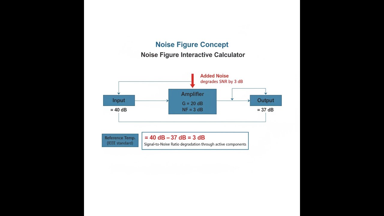
Noise figure is a number — in decibels — that tells you how much worse the signal-to-noise ratio gets as a signal passes through a device like an amplifier or mixer. A noise figure of 0 dB means the device adds no noise at all. A noise figure of 3 dB means the SNR at the output is half what it was at the input.
Simple Explanation
Think of a radio signal as a voice message being passed down a line of people. Each person whispers it to the next, but also adds a little of their own background muttering. Noise figure measures how much muttering each person adds relative to the original message. The quieter the first person in line, the better — because everyone else's muttering gets drowned out by the time the message is amplified.
📐 Browse all 1000+ Interactive Calculators
System Diagram

How to Use This Calculator
- Select a calculation mode from the dropdown — choose from noise figure from SNR, cascaded NF, output SNR, or noise temperature conversion.
- Enter your known values into the input fields shown for that mode — SNR values in dB or linear, stage noise figures in dB, stage gains in dB, or noise temperature in Kelvin.
- Check that all fields are filled with valid numbers before proceeding.
- Click Calculate to see your result.
Interactive Noise Figure Calculator
Noise Figure Interactive Visualizer
Watch how noise figure cascades through amplifier stages and see the critical importance of first-stage design. Adjust stage gains and noise figures to understand why low-noise amplifiers cost more than all subsequent stages combined.
TOTAL NF
1.81 dB
STAGE 2 CONTRIB
0.31 dB
TOTAL GAIN
35 dB
FIRGELLI Automations — Interactive Engineering Calculators
Equations & Variables
Use the formula below to calculate noise figure from the ratio of input to output signal-to-noise ratio.
Noise Figure Definition
F = SNRin / SNRout
NF = 10 log10(F) = SNRin,dB − SNRout,dB
Use the formula below to calculate cascaded noise figure for a two-stage receiver chain.
Friis Cascade Formula (Two Stages)
Ftotal = F1 + (F2 − 1) / G1
Use the formula below to calculate cascaded noise figure across N stages.
Friis Cascade Formula (N Stages)
Ftotal = F1 + (F2 − 1) / G1 + (F3 − 1) / (G1G2) + ...
Use the formula below to calculate noise figure from equivalent noise temperature.
Noise Temperature Relationship
F = 1 + Te / T0
Te = T0(F − 1)
Variable Definitions
- F — Noise factor (dimensionless linear ratio)
- NF — Noise figure (dB), always NF = 10 log10(F)
- SNRin — Signal-to-noise ratio at the input (linear or dB)
- SNRout — Signal-to-noise ratio at the output (linear or dB)
- Gn — Power gain of stage n (linear ratio or dB)
- Fn — Noise factor of stage n (linear ratio)
- Te — Equivalent noise temperature (Kelvin)
- T0 — Reference temperature, IEEE standard = 290 K
Simple Example
An amplifier receives a signal with an input SNR of 30 dB and outputs it at 27 dB SNR.
NF = SNRin − SNRout = 30 − 27 = 3 dB
Linear noise factor F = 10^(3/10) = 2.0 — the amplifier doubles the noise relative to the signal.
Theory & Practical Applications
Fundamental Noise Theory and the Physical Origins of Noise Figure
Noise figure quantifies how much a device degrades the signal-to-noise ratio of a signal passing through it. Unlike gain or bandwidth, which directly affect signal amplitude or frequency response, noise figure captures the less intuitive phenomenon of how thermal agitation in resistors, shot noise in semiconductors, and flicker noise in transistors contaminate signals with random fluctuations. Every active device adds noise to the signal, and this addition is fundamentally different from passive attenuation—it cannot be reversed by subsequent amplification without also amplifying the added noise.
The reference temperature T₀ = 290 K (16.85°C) used in the IEEE standard is not arbitrary. It represents a practical room-temperature approximation for terrestrial communications systems. At this temperature, thermal noise power in a 1 Hz bandwidth is kT₀ ≈ −174 dBm/Hz, where k is Boltzmann's constant (1.38 × 10⁻²³ J/K). This establishes the baseline against which all noise contributions are measured. A device with NF = 3 dB effectively adds noise power equal to doubling the thermal noise floor—equivalent to raising the input temperature by 290 K.
A critical non-obvious insight: noise figure is not a measure of total noise at the output—it is a measure of noise added by the device relative to the noise already present at the input. A high-gain amplifier with NF = 6 dB can have lower absolute output noise than a low-gain amplifier with NF = 2 dB if the input noise is sufficiently low. This distinction becomes crucial in system design when cascading stages with different gains and noise figures. The Friis formula reveals that the first stage dominates system noise performance: subsequent stages contribute noise divided by the cumulative gain of all preceding stages.
Cascaded Noise Figure and the Critical Role of First-Stage Design
The Friis cascade formula, F_total = F₁ + (F₂ − 1)/G₁ + (F₃ − 1)/(G₁G₂) + ..., is the most important equation in RF front-end design. It shows that the noise contribution of the second stage is reduced by the gain of the first stage, the third stage's contribution is reduced by the product of the first two gains, and so on. This creates an exponential decay in the importance of later stages. In a satellite receiver with a first-stage LNA providing 20 dB gain (G₁ = 100 linear) and NF₁ = 0.8 dB (F₁ = 1.202), even a second-stage mixer with NF₂ = 8 dB (F₂ = 6.31) contributes only (6.31 − 1)/100 = 0.0531 in linear terms, or approximately 0.22 dB to the total system noise figure.
This mathematical reality drives the economics of receiver design: spending extra budget on a low-noise first-stage amplifier with NF = 0.5 dB instead of NF = 1.5 dB can reduce system noise figure by 1 dB, which translates to 26% improvement in receiver sensitivity (1 dB ≈ 1.26×). The same 1 dB improvement in the third stage would contribute less than 0.01 dB to system performance if preceded by two stages with 15 dB gain each. This is why low-noise amplifiers (LNAs) in cellular base stations often cost more than all subsequent stages combined.
An edge case that catches designers: passive components like cables, filters, and switches before the first amplifier stage are catastrophic for noise figure. A cable with 3 dB loss (50% power attenuation) has NF = 3 dB, but more critically, it appears before any gain, so its contribution is not reduced by the Friis formula. A system with a perfect amplifier (NF = 0 dB) preceded by a 3 dB cable will have system NF = 3 dB. This is why satellite dishes place the LNA directly at the antenna feed, minimizing cable length between antenna and amplifier to fractions of a meter, even though this complicates installation and maintenance.
Real-World Applications Across Communication Systems
In 5G millimeter-wave base stations operating at 28 GHz or 39 GHz, noise figure dominates link budget calculations because path loss scales with frequency squared. A 39 GHz signal experiences 22 dB more path loss than a 2.4 GHz signal over the same distance. With such aggressive path loss, every 0.1 dB of noise figure improvement translates to meters of additional coverage radius or the difference between achieving 100 Mbps versus 50 Mbps at the cell edge. Modern GaN HEMT amplifiers achieve NF below 2 dB at these frequencies, but maintaining this performance across temperature variations from −40°C to +85°C requires careful bias circuit design and temperature compensation.
Radar receivers face unique noise figure challenges because they must detect echoes 100 dB weaker than the transmitted pulse. A marine radar operating at 9.4 GHz with 25 kW peak transmit power must detect returns at −90 dBm while the transmitter leakage and passive reflections can be −20 dBm. The receiver's noise figure directly determines the maximum detection range via the radar equation: doubling the range requires 12 dB more sensitivity (fourth-power law), which corresponds to improving NF by 12 dB—impossible without fundamental technology changes. Instead, designers use time-gating to turn off the receiver during transmit pulses and employ ferrite circulators with 30+ dB isolation to prevent transmitter noise from desensitizing the receiver.
Radio astronomy represents the ultimate noise figure challenge. Detecting cosmological signals at wavelengths where the cosmic microwave background contributes only −200 dBm/Hz (equivalent to 2.7 K antenna temperature) requires cryogenically cooled amplifiers operating at 4 K to achieve system noise temperatures below 10 K (NF ≈ 0.15 dB). These High Electron Mobility Transistor (HEMT) amplifiers use liquid helium cooling and InP (indium phosphide) semiconductors to minimize 1/f noise. The Square Kilometre Array (SKA) project uses 131,072 antennas each with sub-20 K system temperature to achieve sensitivity capable of detecting airport radar signals on exoplanets 50 light-years away.
Worked Multi-Part Example: Satellite Ground Station Receiver Design
Scenario: Design a Ku-band satellite downlink receiver (12.4 GHz) for receiving data at 50 Mbps with BER = 10⁻⁶. The system comprises: (1) antenna with 45 dBi gain and 55 K system temperature, (2) 15 meters of LMR-600 coaxial cable, (3) low-noise amplifier, (4) mixer, and (5) IF amplifier. Satellite EIRP = 52 dBW, range = 38,500 km, required C/N₀ = 58 dB-Hz for the modulation scheme.
Part A: Calculate received signal power at antenna terminals
Free-space path loss at 12.4 GHz over 38,500 km:
FSPL = 20 log₁₀(4πd/λ) where λ = c/f = 3×10⁸ / 12.4×10⁹ = 0.0242 m
FSPL = 20 log₁₀(4π × 3.85×10⁷ / 0.0242) = 20 log₁₀(1.996×10¹⁰) = 206.0 dB
Received power: P_rx = EIRP + G_antenna − FSPL
P_rx = 52 dBW + 45 dBi − 206.0 dB = −109.0 dBW = −79.0 dBm
Part B: Determine cable loss and noise contribution
LMR-600 cable attenuation at 12.4 GHz: 8.2 dB per 100 feet = 0.269 dB/m
For 15 m: Loss = 15 × 0.269 = 4.04 dB
Cable noise figure: NF_cable = Loss = 4.04 dB (a passive lossy component has NF equal to its loss)
Signal power after cable: −79.0 dBm − 4.04 dB = −83.04 dBm
Part C: Calculate required system noise figure for C/N₀ specification
Thermal noise power: N₀ = kT₀ = −174 dBm/Hz at T₀ = 290 K
Required carrier-to-noise density: C/N₀ = 58 dB-Hz
Required noise density: N₀_system = P_rx − C/N₀ = −83.04 dBm − 58 dB = −141.04 dBm/Hz
System noise figure: NF_system = N₀_system − (−174 dBm/Hz) = −141.04 − (−174) = 32.96 dB
This seems very high and indicates the system is noise-limited by the cable loss appearing before amplification.
Part D: Design amplifier chain to minimize system noise figure
Select components:
• LNA: NF₁ = 0.7 dB (F₁ = 1.175), G₁ = 22 dB (G₁ = 158.5 linear)
• Mixer: NF₂ = 7.5 dB (F₂ = 5.623), G₂ = −6 dB (conversion loss, G₂ = 0.251 linear)
• IF Amp: NF₃ = 3.5 dB (F₃ = 2.239), G₃ = 30 dB (G₃ = 1000 linear)
Cascaded noise figure (after cable):
F_total = F— + (F₂ − 1)/G₁ + (F₃ − 1)/(G₁ × G₂)
F_total = 1.175 + (5.623 − 1)/158.5 + (2.239 − 1)/(158.5 × 0.251)
F_total = 1.175 + 0.02916 + 0.03115 = 1.235
NF_total = 10 log₁₀(1.235) = 0.917 dB
System noise figure including cable (using cable as first stage with G_cable = 0.395):
F_system = F_cable + (F_amplifiers − 1)/G_cable
F_system = 2.535 + (1.235 − 1)/0.395 = 2.535 + 0.595 = 3.130
NF_system = 10 log₁₀(3.130) = 4.95 dB
System noise density: N₀_actual = −174 dBm/Hz + 4.95 dB = −169.05 dBm/Hz
Achieved C/N₀ = −83.04 dBm − (−169.05 dBm/Hz) = 86.01 dB-Hz
Conclusion: The design exceeds requirements by 28 dB, providing substantial link margin. The 4 dB cable loss costs 4 dB in system noise figure but is unavoidable in this geometry. Moving the LNA to the antenna feed (weatherproof enclosure) would reduce cable loss to near zero and improve system NF to 0.92 dB, gaining 4 dB link margin—equivalent to doubling transmit power or quadrupling data rate.
Practical Measurement Techniques and Common Pitfalls
Measuring noise figure below 1 dB requires specialized instruments and careful technique. The Y-factor method uses a calibrated noise source that switches between hot (T_hot ≈ 7000 K) and cold (T_cold = 290 K) states while measuring output power. The noise figure is computed from F = (T_hot − Y×T_cold)/(T_cold(Y − 1)), where Y is the ratio of hot to cold output powers. Measurement accuracy degrades rapidly for NF below 0.5 dB because the Y-factor approaches unity, making small measurement errors dominate the result. Vector network analyzers (VNAs) with noise figure measurement options achieve 0.1 dB accuracy by using multiple calibration standards and averaging thousands of measurements.
A common error: measuring noise figure with insufficient termination bandwidth. If the termination (typically a 50Ω load) has reactive components that vary across the measurement bandwidth, the measured noise temperature varies with frequency, creating artifacts in the NF measurement. High-quality loads use tapered resistive films and maintain VSWR below 1.2:1 (return loss > 20 dB) across decades of bandwidth. Temperature stabilization is also critical—a 1°C change in ambient temperature shifts measured NF by approximately 0.01 dB for a 3 dB noise figure device.
Frequently Asked Questions
Free Engineering Calculators
Explore our complete library of free engineering and physics calculators.
Browse All Calculators →🔗 Explore More Free Engineering Calculators
- LED Resistor Calculator — Current Limiting
- Capacitor Charge Discharge Calculator — RC Circuit
- I2C/SPI Bus Speed & Pull-up Resistor Sizing
- RLC Circuit Calculator — Resonance Impedance
- J Pole Antenna Calculator
- Series Inductors Calculator
- Parallel Capacitor Calculator
- Ohm's Law Calculator — V I R P
- Wire Gauge Calculator — Voltage Drop AWG
- Voltage Divider & ADC Resolution Calculator
About the Author
Robbie Dickson — Chief Engineer & Founder, FIRGELLI Automations
Robbie Dickson brings over two decades of engineering expertise to FIRGELLI Automations. With a distinguished career at Rolls-Royce, BMW, and Ford, he has deep expertise in mechanical systems, actuator technology, and precision engineering.
Need to implement these calculations?
Explore the precision-engineered motion control solutions used by top engineers.


