Modulation Interactive Calculator

If you're designing a radio link or wireless system, you need to pay close attention to how your signal takes up spectrum. Miss the mark and you’ll end up wasting power, running into regulatory problems, or degrading your signal-to-noise ratio. This Modulation Interactive Calculator is laid out for practical use: you can quickly calculate modulation depth, bandwidth, sideband locations, deviation ratios, and how power splits between carrier and sidebands in AM, FM, or PM. These are the actual calculations that show up in radio, telemetry, and broadcast work—not just in textbooks, but on the bench and in the field. Scroll down for the key formulas, a real-world FM transmitter design, direct technical explanations, and answers to typical engineering questions.

What is modulation?

Modulation means you take a basic carrier wave (usually a sine wave at high frequency) and change its amplitude, frequency, or phase according to whatever information you want to transmit. This process makes signals travel much further and lets you use sensible antennas and standard receivers.

Simple Explanation

The carrier is just a base signal until you put information onto it. If you use amplitude modulation (AM), you’re making the wave bigger or smaller as your signal changes. With frequency modulation (FM), the carrier speeds up or slows down, but doesn't get "taller". Phase modulation (PM) shifts the carrier forward and backward in time. Each method trades off noise resistance, bandwidth requirements, and hardware needs. None is universally better—what’s best depends on your constraints.

📐 Browse all 1000+ Interactive Calculators

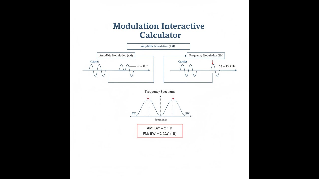
Modulation Diagram

How to Use This Calculator

1. Pick the modulation parameter you want to solve for: AM depth, AM power, AM bandwidth, FM deviation, FM index, or PM index.
2. Enter the appropriate values—make sure to match the variable names with your calculation (for example, amplitudes in volts for AM depth, frequency deviation and modulating frequency for FM index).
3. Use the right units for each field: Hz for frequency, volts for amplitude, watts for power.
4. Click Calculate, and review the answer and anything else the tool flags for your input set.

Modulation Interactive Calculator

Modulation Equations

The following formulas get you to modulation depth, how the power gets divided, and what bandwidth to expect in AM.

These are the working equations for FM deviation, index, and bandwidth. Good enough for most real life cases.

Use the following if you’re working with phase modulation directly.

Simple Example

FM modulation index calculation:

• Frequency deviation (Δf): 75,000 Hz
• Modulating frequency (f_m): 15,000 Hz
• Modulation index: β = 75,000 / 15,000 = 5.000
• Bandwidth (Carson's Rule): 2 × (75,000 + 15,000) = 180 kHz

Theory & Practical Applications

Fundamental Principles of Modulation

Modulation is just the process of varying a carrier’s key property—amplitude, frequency, or phase—so that the information signal “rides along” for transmission. Without this step, long distance transmission would need impractically large antennas, especially for low-frequency (audio) signals. Modulation lets you shift your signal to higher frequencies where standard antennas and filtering become feasible, and it’s the reason spectrum can be divvied up for multiple users by frequency.

No one uses a 10 km wire antenna for a 30 Hz signal. If you try, most of your power gets lost as heat or radiated in unwanted directions. Modulation pushes the message up to radio frequencies (RF), turning a physics problem into a manageable one.

Amplitude Modulation: Analysis & Limitations

For AM, the carrier amplitude is changed in step with the baseband signal. The math is dead simple for a single tone: you end up with one carrier and two symmetric sidebands. But there’s a catch—let modulation depth m creep above 1 and the waveform actually tries to invert, which it can’t do in reality, resulting in flat-topped “clips” and a noisy, splattery spectral output. This is an easy way to blow past emission limits and get your signal rejected by basic receivers.

One problem with classic AM is that most of your transmitter power—up to two thirds—serves no purpose except keeping things compatible with cheap receivers. Only one third of the power goes into the actual sidebands that hold the information. SSB and similar schemes solve this by removing the carrier and one sideband entirely, but require a more capable receiver with extra oscillator circuits or DSP.

Frequency Modulation: Carson's Rule & Deviation Ratio

FM works by swinging the carrier’s frequency back and forth based on your modulating signal. The amount you swing it—the deviation—sets your modulation index. Narrowband FM (NBFM) behaves a lot like AM in terms of bandwidth, but wideband FM goes the other direction: the number of sidebands multiplies with modulation index and the spectrum gets crowded. That’s why FM radio takes much more space on the dial than AM.

Use Carson’s rule to estimate how much bandwidth you’ll need: about twice the sum of deviation and the modulating frequency. It’s not exact, but in nearly all communication system design it’s practical and gets you into regulatory compliance. If you let the modulation index get very large, theoretically your sidebands march on forever, but signal power is concentrated in just a handful set by the index. In practice, limiting the deviation (and index) keeps things sane and neighboring users happy.

FM’s big advantage over AM is its immunity to amplitude noise, but only above a certain carrier-to-noise threshold. Below that, the signal can fall apart quickly (threshold effect). Above threshold, you get a noise performance that scales with the square of your modulation index, a huge reason why FM is favored for clean audio and robust industrial telemetry.

Phase Modulation & Relationship to FM

Phase modulation is like FM but with a twist—you directly shift the phase of the carrier, rather than its frequency. For a simple sinewave, PM and FM look basically the same, but for more complex or wideband signals, their main difference is how phase and frequency deviation depend on message frequency. PM is naturally used in many digital schemes (like PSK) since phase changes are easy to match to data transitions, and phase-only modulation is easier to generate cleanly at high rates.

In both FM and PM designs, think through the relationship between deviation, message bandwidth, and what your receiver can track. FM demodulation is generally done by frequency discriminators (analog or digital). PM systems often use similar detectors but might need differentiation or integration before and after.

Worked Example: FM Transmitter Design for Industrial Telemetry

Take a real case: a temperature sensor gives 0-5 V representing 0-100°C and you want to transmit that over a 433.92 MHz radio channel, using no more than 150 kHz of spectrum (to avoid spillage into neighboring ISM devices). The sensor is slow—it never changes faster than 50 Hz.

Step 1: Work out your deviation. Carson’s rule gives you bandwidth as 2(Δf + f_m), so Δf = [BW/2] - f_m = 75,000 Hz. That’s your max shift up or down from the carrier center.

Step 2: Modulation index? β = 75,000 / 50 = 1500. You’ll get a ridiculous number of sidebands for a single tone—wider than you’ll ever use in real voice or telemetry.

Step 3: Set frequency sensitivity. For maximum sensor output (5 V, 100°C), k_f = 75,000 Hz / 5 V = 15,000 Hz/V. Set up your VCO accordingly.

Step 4: Map the output. Zero volts (0°C) puts you 75 kHz below center (433.845 MHz), 5 V (100°C) moves you 75 kHz above. The channel fits cleanly inside the ISM band for 433 MHz radios.

Step 5: How many useful sidebands? Theoretically, about n = β + 1, so around 1501. For practical purposes, though, you’re mainly interested in the 150 kHz occupied bandwidth.

Step 6: Discriminator setup. For full sensor swing (5 V) and 150 kHz deviation, set your output conversion to about 33.3 μV/Hz, and make sure the bandwidth of your phase-locked loop or frequency discriminator easily tracks the 0-50 Hz temperature changes.

Step 7: Any pre-emphasis needed? Not here—the signal starts at DC. Pre-emphasis only matters for signals that roll off at the low end (like voice or audio). The high deviation ratio already gives you SNR well above what’s needed for typical industrial noise.

Applications Across Industries

Telecommunications: Medium-wave and shortwave radio stick with AM since the propagation supports long range (especially at night). SSB is used when you want to save both power and bandwidth—important in HF comms. For local mobile radio, NBFM is favored because you can get the benefits of FM’s noise rejection without hogging spectrum, provided your messages are fairly narrowband (speech, telemetry).

Broadcasting: FM radio operates wideband for a reason—for 75 kHz deviation and a 15 kHz max audio frequency, you need nearly 200 kHz to avoid adjacent station interference. Stereo, RDS, and subcarriers are layered in as needed, each with their own practical deviation limits. Analog TV mixes AM (for video) and FM (for audio), but that’s giving way to all-digital modulation schemes that maximize spectral efficiency with QAM-style approaches.

Instrumentation & Telemetry: Sensors often get their output modulated onto a low-frequency carrier to reject drift and low-frequency noise in analog lines, or ride as analog channels in multi-channel FM telemetry systems especially in aerospace—where robust, simple, and parallel signaling is more important than squeezing every dB of bandwidth. More systems are heading digital with PCM/FM, but analog FM is still widely used for legacy and certain environments.

Radar & Navigation: FM and PM-based techniques dominate in Doppler and FMCW radar. These methods allow direct measurement of speed and range by monitoring frequency shifts, and the resilience to environmental noise is crucial. Modern navigation like GPS goes for phase-based digital modulation for its precision and sensitivity.

Advanced Design Considerations

There’s never a perfect modulation scheme. AM is simple but burns transmitter power. FM and PM substantially improve noise performance and power efficiency in constant envelope systems (letting you use higher-efficiency power amps), at the cost of more bandwidth and circuit complexity. Hardware makes a difference—push-pull and class C amplifiers are quite efficient in FM/PM, but distort AM badly. Each effect shows up clearly on the bench. Digital radios further complicate things, since high-speed DACs, IQ bases, and quantization noise start to dictate system constraints. Your real bottlenecks are often regulatory, hardware, and antenna choices, not just “which modulation is best on paper”.

Frequently Asked Questions

Video Walkthrough - How to Use This Calculator