Wave Velocity Interactive Calculator

If you need to work out wave propagation — whether you're sizing an ultrasonic transducer, checking material properties, or calculating seismic travel times — you'll want to know how quickly the wave moves through your chosen medium. With the Wave Velocity Interactive Calculator, you can solve for wave speed, frequency, or wavelength by plugging in relevant values like frequency, wavelength, tension, bulk modulus, or Young’s modulus. This is directly useful in fields like telecom, acoustics, geophysics, NDT, and materials. You'll find the working formulas, a straightforward ultrasonic example, practical propagation notes, and extra FAQ below.

What is wave velocity?

Wave velocity is simply how fast a disturbance — sound, vibration, or electromagnetic — gets from one place to another in a material or medium. The speed depends on the physical makeup of the medium, not on the disturbance's size or strength.

Simple Explanation

Picture wave velocity like passing along a message in a crowded room. How fast it spreads depends on how tightly packed and attentive everyone is, not how loud the starting shout was. In something like steel, where atoms are closely linked, waves race along because each push transfers quickly down the line. In air, atoms are far apart and loosely interacting, so the wave crawls along comparatively slowly.

📐 Browse all 1000+ Interactive Calculators

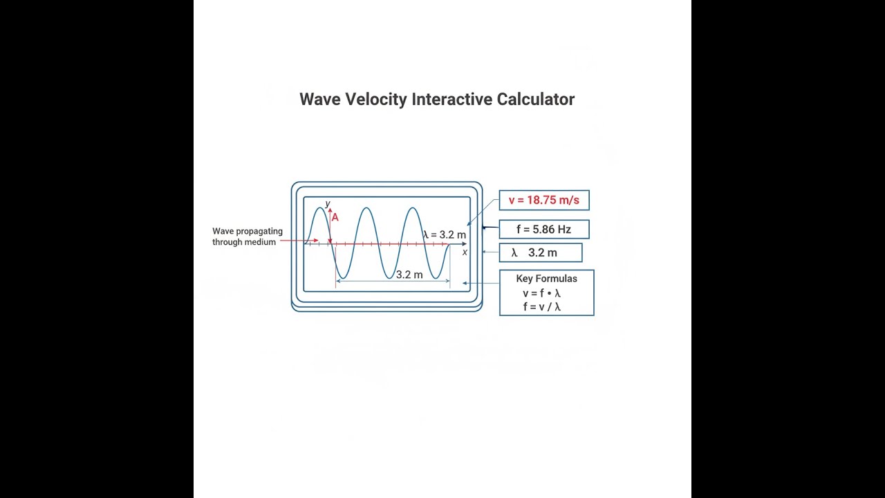
Wave Propagation Diagram

Interactive Wave Velocity Calculator

How to Use This Calculator

1. Pick a Calculation Mode from the dropdown — you’ll usually know if you’re solving for frequency/wavelength, or you have a problem involving string tension, or you’ve got a bulk or Young’s modulus from your material data.
2. Enter relevant numbers in the boxes for your chosen mode — frequency in Hz and wavelength in meters, or tension in newtons and linear density in kg/m, as appropriate.
3. Double-check your units. The calculator assumes SI units (meters, Newtons, Pascals, kg/m³).
4. Click Calculate to see the result.

<> Embed this calculator → <> Embed this animation calculator →

Wave Velocity Equations

You can use this formula to get wave velocity from frequency and wavelength.

If you’re working with a stretched string, use this formula:

For sound waves in a fluid, use this formula:

If you’re looking at longitudinal waves in a rod, here's what you need:

Simple Example

Suppose a sound wave in air has a frequency of 500 Hz and a wavelength of 0.686 m. Using v = f × λ: v = 500 × 0.686 = 343 m/s. That lines up with the typical speed of sound in air at 20°C. The period is 1/500 = 0.002 s, and the wave number is 2π/0.686 = 9.16 rad/m.

Theory & Practical Applications

Fundamental Physics of Wave Propagation

Wave velocity is just the speed at which a disturbance travels through a medium; it’s not the same as the speed of the particles themselves. For mechanical waves, it boils down to two things: the restoring force (think elastic modulus or string tension—how hard the material works to get back to its original position) and the inertia (density or mass per meter, which resists that recovery). That’s why in practice, all these wave speed formulas come down to the square root of stiffness over inertia.

The link v = fλ is simple but important: in a given medium, if you crank up the frequency, the wavelength gets shorter. Push it down, and the wavelength gets longer. This ties directly into real choices — if you want precise ultrasonic images, you need a higher frequency (shorter λ), but that might make the waves more prone to attenuation. Medium properties set the limit; as soon as you encounter a different material or nonlinear effect, the simple formula no longer tells the whole story.

String Wave Mechanics and Musical Instruments

For a vibrating string, the key formula is v = √(T/μ). Here, μ (linear mass density) isn't just density, it’s mass per length, so not only material but string thickness and construction matter — identical-diameter nylon and steel strings behave very differently. In practice, instrument tuning is about adjusting tension T while keeping μ and length set by the instrument. If you want a lower pitch, you usually pick a thicker string; dropping the tension too much fast runs into instability or buzzing.

You also run up against the strength limits of your materials pretty quickly. Take a steel string: 1 mm diameter, 650 mm long gives μ ≈ 0.005 kg/m. To get standard A440 (wavelength 1.3 m) you need v ≈ 572 m/s, which in turn demands a tension of about 1640 N. That pushes the stress close to 2 GPa, about 80% of the yield strength for quality music wire. This is why pianos—where string forces add up quickly—use beefy frames and multiple strings per note to stay within mechanical limits.

Sound Propagation in Fluids and Gases

Wave speed in fluids is set by the bulk modulus (how hard the fluid is to compress). Water’s high modulus means waves travel fast—around 1480 m/s. In air, the much lower modulus drops speed to 343 m/s. This major speed jump is why sonar travels well underwater, and why designing acoustic devices for air vs. water requires different inputs.

Temperature affects air sound speed most by changing its density. For everyday practical estimates, air sound speed goes up about 0.6 m/s for each °C rise in temperature. This is enough to bend sound as it travels (causing the well-known temperature inversion sound “carry” at night). Humidity’s effect is smaller but visible in metrology, as water vapor is lighter than dry air and nudges speed up by a few m/s at high humidity.

Elastic Waves in Solids and Seismic Applications

Solids support a few wave types: P-waves (longitudinal), S-waves (shear), and various surface waves. The speed for each depends on the material elastic properties and geometry — rods and wires are handled with the simple v = √(E/ρ), but full 3D solids need bulk and shear modulus together in the formulas. For most steels, you get around 5000 m/s for P-waves and 3000 m/s for S-waves. This speed difference is crucial in seismology, where it’s used for earthquake epicenter location by timing the P and S-wave arrivals. The math is direct distance = velocity × time, using practical velocities from your region’s geology.

Worked Example: Ultrasonic Testing Transducer Design

Problem: An ultrasonic testing technician plans to check a steel vessel with a 5 MHz longitudinal probe. Steel data: ρ = 7850 kg/m³, E = 207 GPa. The probe’s spatial resolution is about half the wavelength. Figure out: (a) wave velocity in steel, (b) wavelength at 5 MHz, (c) smallest detectable crack, (d) round-trip time through a 150 mm wall, (e) frequency needed for 0.25 mm cracks.

Solution:

Part (a): For steel, v = √(E/ρ): v = √(207 × 10⁹ / 7850) = √(26,369,426.75) ≈ 5135 m/s.

Part (b): At 5 MHz: λ = v/f = 5135 / (5 × 10⁶) = 1.03 × 10⁻³ m ≈ 1.03 mm.

Part (c): Resolution is roughly λ/2: 1.03 mm / 2 ≈ 0.51 mm. This is the smallest crack this probe could “see.”

Part (d): Time for echo through 150 mm wall and back: distance = 0.3 m, so time = 0.3 / 5135 ≈ 58 μs for round trip.

Part (e): If you want 0.25 mm cracks, target λ = 0.5 mm, so need f = 5135 / 0.0005 = 10.3 MHz. So a 10 MHz (or greater) probe.

Engineering Implications: In real inspection jobs, you can’t just crank frequency endlessly — higher frequencies make waves easier to block or attenuate, especially in thick or dirty steel. The 5 MHz probe offers a usable compromise between resolution and how deep the signal can go. Small, near-surface flaws sometimes justify 10–15 MHz probes, but for thick sections you’ll likely use 1–5 MHz. The echo time gives you not just flaw detection but also wall thickness, which is useful for jobs like corrosion checks in industrial tanks.

Dispersion and Frequency-Dependent Velocity

The basic v = fλ assumes the speed doesn’t change with frequency. But in a lot of real cases, especially for waves in water or on surfaces, different frequencies travel at different speeds (dispersion). You see this in ocean waves: long swells outpace short wind chop. In optics, it means different colors (wavelengths) travel differently through glass, which causes pulse spreading in fiber links. When calculating pulse spread, the main practical concern is picking a fiber or a frequency region with minimal dispersion near your operating point. For single-mode telecom fiber, zero-dispersion is targeted around 1550 nm, but any spectral width will still create a bit of pulse broadening over long runs, setting data rate limits and the need for compensation schemes.

Industrial Applications and Measurement Techniques

Engineers use wave velocity to characterize materials without cutting them open. You can measure both longitudinal and shear velocities in a sample and then back out elastic constants. Useful benchmarks include tracking concrete cure with time (velocity rises as the matrix strengthens) or watching for freeze-thaw issues (velocity falls in damaged pavement). In machinery, a drop in ultrasonic velocity could point to forming cracks or other kinds of fatigue before failure.

Ultrasonic flow meters compare travel times upstream and downstream; the speed difference gives fluid velocity. For water pipes with transducers at a known angle and spacing, a difference of a few hundred nanoseconds in time is enough for a complete flow reading with only moderate electronics.

There are more calculators for specialized wave behaviors and electromagnetic design at the engineering calculator hub.

Frequently Asked Questions

Video Walkthrough - How to Use This Calculator