Diffraction Interactive Calculator

This interactive diffraction calculator analyzes wave behavior when passing through apertures or around obstacles, computing angular positions of minima and maxima for single-slit, double-slit, and diffraction grating configurations. Diffraction patterns govern the resolution limits of optical instruments from microscopes to telescopes, define the performance boundaries of fiber optic systems, and determine the spectral resolution of scientific spectrometers used in materials analysis and astronomy.

📐 Browse all free engineering calculators

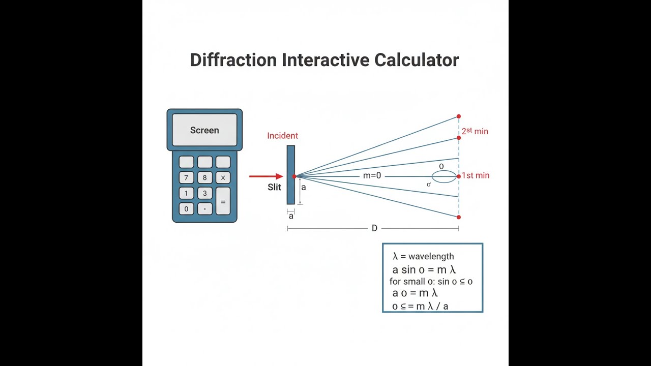
Diffraction Pattern Diagram

Diffraction Calculator

Governing Equations

Theory & Practical Applications

Physical Origins of Diffraction

Diffraction represents the departure of wave propagation from the straight-line predictions of geometric optics. When wavefronts encounter an aperture, edge, or obstacle with dimensions comparable to the wavelength, Huygens' principle dictates that every point on the unobstructed portion of the wavefront acts as a source of secondary spherical wavelets. The superposition of these wavelets produces the observed diffraction pattern — an interference effect arising from the coherent addition of waves traveling different path lengths to any observation point.

For single-slit diffraction, the key insight is that light from different portions of the slit arrives at off-axis observation points with varying phase relationships. When the slit width a and observation angle θ satisfy a sin(θ) = mλ (where m is an integer), light from the top half of the slit interferes destructively with light from the bottom half, producing a minimum. The central maximum spans from m = -1 to m = +1 and contains approximately 95% of the total diffracted energy. This intensity concentration explains why single-slit patterns appear much brighter at center than at the fringes — a critical consideration in optical power budgeting for laser beam delivery systems.

The transition from Fraunhofer (far-field) to Fresnel (near-field) diffraction occurs when the Fresnel number F = a²/(λL) approaches unity, where L is the observation distance. Fraunhofer conditions (F much less than 1) are assumed in most engineering calculations because they simplify to angular analysis, but precision optical systems operating at short working distances must account for Fresnel effects where the phase contributions from different aperture zones no longer reduce to simple angular relationships.

Resolution Limits in Optical Instruments

The Rayleigh criterion defines the fundamental diffraction-limited resolution of imaging systems. For a circular aperture of diameter D observing at wavelength λ, the angular radius of the Airy disk (the central diffraction spot) is θ = 1.22λ/D radians. Two point sources are considered "just resolved" when the central maximum of one Airy pattern coincides with the first minimum of the other. This is not a hard physical boundary — the Sparrow criterion and other definitions exist — but the Rayleigh criterion provides a conservative, widely-adopted standard.

For visible light (λ ≈ 550 nm) and the human eye's 7 mm dark-adapted pupil, the diffraction limit is approximately 1 arcminute (0.29 mrad). In practice, atmospheric turbulence and ocular aberrations degrade resolution to roughly 1 arcminute under good conditions, making the eye nearly diffraction-limited for photopic vision. This explains why astronomical observations benefit enormously from large-aperture telescopes: doubling the aperture halves the Airy disk radius, quadrupling the resolving power. The Hubble Space Telescope's 2.4 m primary mirror achieves 0.05 arcsecond resolution at 500 nm wavelength — approximately 100 times better than ground-based instruments fighting atmospheric seeing.

Microscope resolution follows the same physics but inverts the geometry. The Abbe diffraction limit for a microscope objective with numerical aperture NA = n sin(α), where n is the refractive index of the medium and α is the half-angle of the acceptance cone, gives lateral resolution d = 0.61λ/NA. High-NA oil-immersion objectives (NA ≈ 1.4) achieve d ≈ 200 nm for green light, defining the "diffraction barrier" that limited optical microscopy for over a century. Super-resolution techniques (STED, PALM, STORM) circumvent this limit through clever manipulation of fluorophore emission states, but the underlying diffraction physics remains unchanged.

Diffraction Gratings in Spectroscopy

Diffraction gratings disperse polychromatic light by wavelength through constructive interference at discrete angles satisfying d sin(θ) = mλ. Unlike prisms, which disperse via wavelength-dependent refractive index, gratings achieve angular separation proportional to wavelength: dθ/dλ = m/(d cos θ). This linear dispersion, combined with the ability to manufacture gratings with thousands of lines per millimeter, makes them indispensable in high-resolution spectroscopy.

The resolving power of a grating — its ability to distinguish two closely-spaced spectral lines — is R = λ/Δλ = mN, where N is the total number of illuminated grooves. A 100 mm wide grating with 1200 lines/mm has N = 120,000 grooves. At second order (m = 2), this yields R = 240,000, sufficient to resolve spectral features separated by Δλ = 550 nm / 240,000 ≈ 2.3 picometers at visible wavelengths. This capability enables precise measurement of Doppler shifts in stellar spectra (velocities of order 1 km/s produce shifts of ~2 pm at 550 nm), isotope identification, and hyperfine structure analysis.

Grating efficiency — the fraction of incident light diffracted into a particular order — depends critically on groove profile. Blazed gratings with asymmetric sawtooth profiles concentrate up to 80% of the light into a single order at the "blaze wavelength" where the groove facet normal bisects the angle between incident and diffracted beams. This efficiency dramatically improves signal-to-noise ratios in spectrometers but introduces wavelength-dependent efficiency curves that must be calibrated. Echelle gratings, operated at high orders (m = 50-150) with coarse groove spacing, achieve extreme angular dispersion for ultra-high-resolution applications like exoplanet radial velocity measurements requiring sub-meter-per-second precision.

Fiber Optic and Waveguide Mode Structure

Single-mode optical fibers exploit diffraction physics to confine light to the fundamental LP₀₁ mode. The normalized frequency parameter V = (2πa/λ)√(n_core² - n_cladding²), where a is the core radius, determines the number of supported modes. Single-mode operation requires V less than 2.405 (the first zero of the Bessel function J₀). For standard telecom fiber at λ = 1550 nm with core radius 4.1 μm and refractive index step Δn ≈ 0.005, V ≈ 2.0, maintaining single-mode behavior.

The mode field diameter (MFD), effectively the diffracting aperture of the fiber, is approximately MFD ≈ 2a(0.65 + 1.619/V^1.5 + 2.879/V⁶) for step-index fiber. At V = 2.0, MFD ≈ 10.4 μm — larger than the physical core. This "tail" extending into the cladding is essential for low-loss fiber splicing: misalignment by 1 μm causes roughly 0.1 dB loss, a critical tolerance in long-haul systems where hundreds of splices accumulate. Multimode fibers with V greater than 10 support hundreds of modes, each with different propagation constants, causing modal dispersion that limits bandwidth to ~500 MHz·km — adequate for short premises networks but catastrophic for long-distance communication.

Antenna Beamwidth and Radio Diffraction

Electromagnetic diffraction governs radio antenna performance identically to optical systems, though wavelength scaling shifts practical designs to dramatically different dimensions. A parabolic dish antenna of diameter D operating at wavelength λ has a diffraction-limited half-power beamwidth θ_3dB ≈ 70λ/D degrees (the numerical coefficient varies slightly with illumination taper). For a satellite TV dish (D = 60 cm) at Ku-band (λ = 2.5 cm), θ_3dB ≈ 2.9°. This tight beam requires precise pointing to maintain signal lock — a 5° azimuthal error moves the beam completely off the geostationary satellite.

Radar systems exploit diffraction limits to determine target angular position. A 3 GHz marine radar (λ = 10 cm) with a 1.8 m horizontal antenna yields θ_azimuth ≈ 3.9° resolution — adequate to separate two ships 680 m apart at 10 km range but insufficient for fine navigation near harbor structures. Higher frequency (X-band, 9 GHz) radar trades atmospheric attenuation for 3× better angular resolution. The cross-range resolution δ_cross = R θ_3dB scales linearly with range R, explaining why space-based SAR (synthetic aperture radar) requires kilometer-scale synthetic apertures to achieve meter-scale ground resolution from orbit.

Comprehensive Worked Example: Spectrometer Design

Problem Statement: Design a Czerny-Turner spectrometer for analyzing Mercury emission lines in the blue-green region. Specifications require resolving the 546.074 nm and 546.227 nm lines (separation Δλ = 0.153 nm) with at least 20% valley depth between peaks. The available diffraction grating has 1200 lines/mm, and the detector array has 50 μm pixel pitch. A 150 mm focal length collimating mirror is budget-constrained. Determine: (a) minimum required diffraction order m, (b) diffraction angle θ for the 546.1 nm doublet center, (c) required number of illuminated grating grooves N, (d) physical grating width W, and (e) linear dispersion at the detector plane.

Solution:

Step 1: Determine required resolving power R. The Rayleigh criterion for resolution requires R = λ/Δλ = 546.1 nm / 0.153 nm = 3569. This is the absolute minimum; 20% valley depth requires approximately R ≈ 1.5 × (λ/Δλ) ≈ 5350 to account for instrumental broadening and finite slit widths. We'll design for R = 6000 to provide margin.

Step 2: Calculate required mN product. Grating resolving power R = mN, so mN = 6000. We must choose an order m that's physically realizable. The grating equation d sin(θ) = mλ limits maximum order to m_max = floor(d/λ). With d = (1 mm)/(1200) = 833.3 nm and λ = 546.1 nm, m_max = floor(833.3/546.1) = 1. First order is the only option before sin(θ) exceeds unity. Therefore m = 1, requiring N = 6000 grooves.

Step 3: Calculate diffraction angle θ. Using d sin(θ) = mλ with m = 1, d = 833.3 nm, λ = 546.1 nm: sin(θ) = (1 × 546.1 nm)/(833.3 nm) = 0.6554. Therefore θ = arcsin(0.6554) = 40.96° = 40°58'.

Step 4: Determine physical grating width W. N = 6000 grooves at 1200 lines/mm spacing requires W = 6000/1200 = 5.0 mm minimum. However, the actual illuminated area depends on beam diameter at the grating. For a Czerny-Turner configuration with f = 150 mm focal length mirrors, a typical entrance slit height of 10 mm will produce a collimated beam diameter of ~12 mm (accounting for aberrations). If the collimated beam underfills the grating, the effective N is proportionally reduced. Assuming the beam diameter matches the grating width, we need W ≥ 5.0 mm, but practical designs use W ≈ 12-15 mm to ensure full illumination. We'll specify W = 12 mm, giving effective N = 1200 lines/mm × 12 mm = 14,400 grooves when fully illuminated, yielding R = 14,400 >> 6000 required. This overdesign provides tolerance for slit width broadening and aberrations.

Step 5: Calculate linear dispersion dℓ/dλ at detector. Angular dispersion is dθ/dλ = m/(d cos θ) = 1/(833.3 nm × cos 40.96°) = 1/(833.3 nm × 0.7548) = 1.590 × 10^-3 rad/nm = 1.590 mrad/nm. At focal length f = 150 mm, linear dispersion is (dℓ/dλ) = f (dθ/dλ) = 150 mm × 1.590 × 10^-3 rad/nm = 0.2385 mm/nm = 238.5 μm/nm. The 0.153 nm doublet separation maps to Δℓ = 0.153 nm × 238.5 μm/nm = 36.5 μm at the detector.

Step 6: Verify detector sampling. With 50 μm pixel pitch, the 36.5 μm doublet separation spans 0.73 pixels — undersampled by the Nyquist criterion. To properly sample the doublet (minimum 2 pixels per line, ideally 3-4), we need pixel pitch ≤ 18 μm or increased focal length f = 150 mm × (50 μm / 18 μm) = 417 mm. Alternatively, accepting the 50 μm pixels with f = 150 mm provides marginal separation but requires deconvolution algorithms to extract line positions. This is a common engineering trade-off: cost of a larger detector array versus complexity of signal processing.

Summary: The spectrometer operates at first order (m = 1) with diffraction angle 40.96°, requires a minimum 5 mm wide grating (12 mm practical), and achieves 238.5 μm/nm linear dispersion. The design marginally resolves the Mercury doublet but is detector-limited, not diffraction-limited, highlighting the crucial interplay between optical design and detector specifications in real spectroscopic systems.

Applications Across Industries

Telecommunications: Wavelength-division multiplexing (WDM) systems use diffraction gratings or arrayed waveguide gratings (AWGs) to combine/separate optical channels spaced 50-100 GHz apart (~0.4-0.8 nm at 1550 nm). Channel crosstalk below -30 dB requires grating resolution R ≈ 2000 and precise temperature control (0.01 nm/°C thermal drift is typical). Dense WDM (DWDM) with 25 GHz spacing pushes requirements to R ≈ 4000.

Astronomy: Adaptive optics systems measure wavefront aberrations using Shack-Hartmann sensors — arrays of lenslets that create diffraction-limited spots whose positions encode local wavefront tilt. Sub-arcsecond imaging requires wavefront sensing at 1 kHz frame rates, with each lenslet aperture sized to produce Airy disks smaller than CCD pixel dimensions. The Extremely Large Telescope (ELT) will employ 6-laser guide stars with 8-meter-class adaptive optics to achieve near-diffraction-limited imaging at visible wavelengths from the ground.

Semiconductor Manufacturing: Photolithography steppers use diffraction to define minimum feature sizes in integrated circuits. The Rayleigh resolution d = k₁λ/(NA), where k₁ ≈ 0.35 for optimized processes, drives the industry toward extreme ultraviolet (EUV) lithography at λ = 13.5 nm. At NA = 0.33 (limited by available EUV optics), this enables d ≈ 14 nm features. Immersion lithography (n = 1.44 for water) extended 193 nm ArF lasers to 38 nm nodes, but further scaling requires shorter wavelengths.

Medical Imaging: Optical coherence tomography (OCT) achieves axial resolution Δz = 2ln(2)λ²/(πΔλ), where Δλ is source bandwidth. Broadband superluminescent diodes (Δλ ≈ 50 nm at λ = 850 nm) provide Δz ≈ 5 μm resolution, enabling cellular-level retinal imaging. Lateral resolution follows standard diffraction limits δ_lateral = 0.61λ/NA, typically 10-20 μm for ophthalmologic systems balancing resolution against working distance and depth of field.

Frequently Asked Questions