Designing a multi-joint robotic arm means knowing exactly where your end effector lands — and with 3 links in the chain, mental math won't cut it. Use this 3-Link Planar Forward Kinematics Calculator to calculate the end effector's X,Y position from 3 link lengths and their respective joint angles. It matters in industrial robotics, surgical device design, and automation systems where workspace accuracy is non-negotiable. This page includes the FK equations, a worked example, application theory, and an FAQ.
What is 3-Link Planar Forward Kinematics?
Forward kinematics is the process of calculating where a robot arm's tip ends up, given the length of each arm segment and the angle at each joint. A 3-link planar system means 3 connected segments all moving in the same flat plane.
Simple Explanation
Think of your arm: your upper arm, forearm, and hand are 3 links. If someone told you the exact angle at your shoulder, elbow, and wrist, you could figure out exactly where your fingertip is in space. That's all forward kinematics does — it translates joint angles into a precise tip position using basic trigonometry.
📐 Browse all 384 free engineering calculators
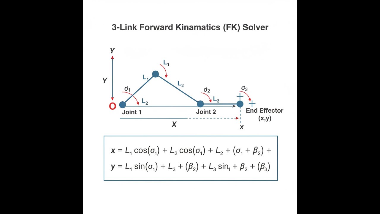
3-Link Planar Arm System Diagram
 Solver | FIRGELLI Engineering Calculator")
3-Link Forward Kinematics Calculator
3-Link Planar Forward Kinematics Interactive Visualizer
Watch how joint angles control your robotic arm's end effector position in real-time. Adjust link lengths and angles to see the kinematic chain solve forward kinematics instantly.
END EFFECTOR X
165 mm
END EFFECTOR Y
128 mm
REACH DISTANCE
209 mm
FIRGELLI Automations — Interactive Engineering Calculators
How to Use This Calculator
- Enter the 3 link lengths (L₁, L₂, L₃) in any consistent unit — mm, inches, or meters.
- Enter the joint angle for each link (θ₁, θ₂, θ₃) in degrees. θ₁ is measured from the positive X-axis; θ₂ and θ₃ are relative to the preceding link.
- Confirm all 6 fields are filled with positive link lengths and valid angle values.
- Click Calculate to see your result.
Mathematical Equations
3-Link Planar Forward Kinematics
Use the formula below to calculate end effector position for a 3-link planar robotic arm.
The forward kinematics equations for a 3-link planar robotic arm are derived using trigonometric relationships and vector addition:
Cumulative Joint Angles:
α₁ = θ₁
α₂ = θ₁ + θ₂
α₃ = θ₁ + θ₂ + θ₃
End Effector Position:
x = L₁ cos(α₁) + L₂ cos(α₂) + L₃ cos(α₃)
y = L₁ sin(α₁) + L₂ sin(α₂) + L₃ sin(α₃)
Reach Distance:
r = √(x² + y²)
Where:
- L₁, L₂, L₃ = Link lengths
- θ₁, θ₂, θ₃ = Joint angles (degrees)
- α₁, α₂, α₃ = Cumulative angles from base frame
- (x, y) = End effector Cartesian coordinates
- r = Distance from origin to end effector
Simple Example
Given: L₁ = 100 mm at θ₁ = 0°, L₂ = 100 mm at θ₂ = 0°, L₃ = 100 mm at θ₃ = 0°
Cumulative angles: α₁ = 0°, α₂ = 0°, α₃ = 0°
x = 100×cos(0°) + 100×cos(0°) + 100×cos(0°) = 300 mm
y = 100×sin(0°) + 100×sin(0°) + 100×sin(0°) = 0 mm
Result: End effector at (300, 0) mm — all links fully extended along the X-axis.
Technical Guide & Applications
Understanding 3-Link Forward Kinematics
The 3-link forward kinematics calculator extends the capabilities of simpler 2-link systems by adding a third degree of freedom, significantly expanding the workspace and dexterity of robotic manipulators. This mathematical framework is fundamental to robotics engineering and forms the basis for trajectory planning, collision avoidance, and precision positioning in automated systems.
Forward kinematics solves the direct geometric problem: given the joint parameters (link lengths and joint angles), determine the position and orientation of the end effector. For a 3-link planar arm, this involves computing the cumulative effect of three rotational joints, each contributing to the final position through trigonometric relationships.
Engineering Principles
The mathematical foundation relies on homogeneous transformation matrices and Denavit-Hartenberg (D-H) parameters. Each link can be represented as a transformation from the previous joint frame, and the forward kinematics problem becomes a series of matrix multiplications. For planar systems, this simplifies to the trigonometric summation shown in our 3-link forward kinematics calculator.
The key insight is that each joint angle affects not only its own link but all subsequent links in the kinematic chain. This coupling is what gives multi-link systems their complexity but also their versatility. The cumulative angle approach accounts for this interdependence by adding each joint angle to all previous joint angles when computing the orientation of each link.
Practical Applications
Industrial Robotics: Manufacturing robots use 3-link (and higher) configurations for assembly operations, welding, and material handling. The additional degree of freedom allows robots to approach targets from multiple orientations while avoiding obstacles.
Medical Devices: Surgical robots and rehabilitation equipment often employ 3-link mechanisms for precise positioning with natural motion profiles that accommodate human anatomy.
Automation Systems: Pick-and-place systems, packaging equipment, and quality inspection systems benefit from the extended reach and flexibility of 3-link configurations. When combined with FIRGELLI linear actuators, these systems can achieve both rotational dexterity and linear extension capabilities.
Worked Example
Consider a 3-link robotic arm with the following specifications:
- Link 1 (L₁): 150 mm, Joint angle (θ₁): 45°
- Link 2 (L₂): 120 mm, Joint angle (θ₂): 30°
- Link 3 (L₃): 80 mm, Joint angle (θ₃): -15°
Step 1: Calculate cumulative angles
- α₁ = 45° = 0.785 rad
- α₂ = 45°— + 30° = 75° = 1.309 rad
- α₃ = 45° + 30° + (-15°) = 60° = 1.047 rad
Step 2: Apply forward kinematics equations
- x = 150°cos(45°) + 120×cos(75°) + 80×cos(60°)
- x = 150×0.707 + 120×0.259 + 80×0.500
- x = 106.1 + 31.1 + 40.0 = 177.2 mm
- y = 150×sin(45°) + 120×sin(75°) + 80×sin(60°)
- y = 150×0.707 + 120×0.966 + 80×0.866
- y = 106.1 + 115.9 + 69.3 = 291.3 mm
Result: The end effector is positioned at (177.2, 291.3) mm from the base origin, with a reach distance of 340.4 mm.
Design Considerations
Workspace Analysis: The 3-link configuration provides a more complex workspace boundary compared to 2-link systems. The workspace includes regions that can be reached with multiple joint configurations (redundancy), which is valuable for obstacle avoidance and joint limit management.
Singularity Management: Kinematic singularities occur when the robot loses degrees of freedom, typically when links become collinear. The 3-link forward kinematics calculator helps identify these critical configurations during design and path planning phases.
Actuator Selection: Each joint requires appropriate actuation, whether through servo motors, stepper motors, or pneumatic systems. For applications requiring linear motion integration, FIRGELLI linear actuators can provide the base translation or end effector extension capabilities.
Advanced Considerations
Dynamic Effects: While forward kinematics focuses on position relationships, real-world systems must account for inertial effects, especially at higher speeds. The mass distribution and moment of inertia of each link affects the dynamic response and control requirements.
Joint Limits: Physical joints have finite rotation ranges, which constrain the effective workspace. The forward kinematics equations remain valid within these limits, but path planning algorithms must ensure joint angles stay within permissible ranges.
Calibration: Manufacturing tolerances in link lengths and joint zero positions affect accuracy. Regular calibration using the forward kinematics model helps maintain positioning precision in production environments.
Integration with Control Systems
Modern robotic systems integrate forward kinematics calculations into real-time control loops. The computational efficiency of the trigonometric approach makes it suitable for embedded controllers running at kilohertz update rates. This enables smooth trajectory following and responsive feedback control.
For automation applications, the 3-link forward kinematics calculator serves as a design verification tool, allowing engineers to validate workspace requirements and optimize link proportions before physical prototyping. This is particularly valuable when integrating with other motion systems, such as linear slides or rotary tables powered by precision actuators.
Frequently Asked Questions
What is the difference between forward and inverse kinematics? ▼
How do I determine the workspace of a 3-link robot arm? ▼
What units should I use for link lengths and angles? —
How does joint coupling affect the motion in 3-link systems? ▼
Can this calculator be used for 3D robotic arms? ▼
What are kinematic singularities and how do I avoid them? ▼
📐 Explore our full library of 384 free engineering calculators →
About the Author
Robbie Dickson
Chief Engineer & Founder, FIRGELLI Automations
Robbie Dickson brings over two decades of engineering expertise to FIRGELLI Automations. With a distinguished career at Rolls-Royce, BMW, and Ford, he has deep expertise in mechanical systems, actuator technology, and precision engineering.
Need to implement these calculations?
Explore the precision-engineered motion control solutions used by top engineers.


