Hydraulic Gradient Interactive Calculator

Designing pipeline systems, drainage networks, or groundwater flow models all hinge on one core parameter — how fast energy is lost along the flow path. Use this Hydraulic Gradient Interactive Calculator to calculate hydraulic gradient, head loss, flow path length, or upstream/downstream head using total head values, flow geometry, and pipe friction inputs. Getting this number right matters in water distribution, environmental remediation, and civil drainage design — an undersized gradient means inadequate flow; an oversized one means erosion or excessive pumping costs. This page covers the governing formulas, a worked example, full theory, and a FAQ.

What is hydraulic gradient?

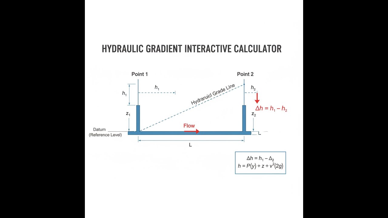
Hydraulic gradient is a dimensionless number that describes how much energy a flowing fluid loses per unit of distance traveled. It equals the drop in total hydraulic head divided by the length of the flow path.

Simple Explanation

Think of hydraulic gradient like the steepness of a water slide — the steeper it is, the faster water moves and the more energy it burns getting from top to bottom. A gentle slope means slow, low-energy flow; a steep slope means fast, high-energy flow. Unlike physical slope, hydraulic gradient accounts for pressure and elevation together, so it works even in pipes running uphill or downhill.

📐 Browse all 1000+ Interactive Calculators

How to Use This Calculator

1. Select your calculation mode from the dropdown — choose what you want to solve for (gradient, head loss, flow path length, upstream or downstream head, or Darcy-Weisbach pipe flow).
2. Enter the upstream hydraulic head (h₁), downstream hydraulic head (h₂), and flow path length (L) in metres — or the relevant inputs for your chosen mode.
3. For the Darcy-Weisbach mode, also enter pipe diameter, flow velocity, and friction factor.
4. Click Calculate to see your result.

Visual Diagram: Hydraulic Gradient in Pipe Flow

Hydraulic Gradient Calculator

Governing Equations

Simple Example

Upstream head h₁ = 10 m, downstream head h₂ = 7 m, flow path length L = 150 m.

Head loss: Δh = 10 − 7 = 3 m

Hydraulic gradient: i = 3 / 150 = 0.02

Slope: 0.02 × 100 = 2%

Theory & Practical Applications

Fundamental Concept and Physical Interpretation

The hydraulic gradient represents the rate of energy dissipation in a flowing fluid system, expressed as a dimensionless ratio of head loss to flow distance. Unlike simple pressure drop, hydraulic gradient incorporates the complete energy state of the fluid — accounting for elevation, pressure, and velocity components through the total hydraulic head. This makes it particularly valuable for analyzing flow in systems with varying elevations or cross-sections, where pressure measurements alone would be misleading.

In groundwater hydrology, the hydraulic gradient governs flow velocity through porous media via Darcy's Law, establishing the direct proportionality between seepage rate and energy gradient. For pipe flow, the gradient quantifies frictional resistance and is essential for pump selection, energy efficiency analysis, and system optimization. The gradient is always positive in the direction of flow (energy decreases downstream), and its magnitude indicates the severity of frictional losses or the natural driving force in gravity-fed systems.

Groundwater and Subsurface Flow Applications

Environmental remediation projects rely heavily on hydraulic gradient calculations to predict contaminant migration rates and design extraction well networks. In a typical pump-and-treat remediation scenario, engineers establish a hydraulic gradient by lowering the water table locally through pumping, creating a cone of depression that captures contaminated groundwater before it reaches sensitive receptors. The required pumping rate depends directly on the induced gradient magnitude and the aquifer's hydraulic conductivity — a relationship that allows optimization of extraction well spacing and flow rates to minimize operational costs while achieving cleanup objectives.

Dewatering operations for construction sites, mining activities, and tunnel excavations must maintain adequate hydraulic gradients to prevent groundwater intrusion. Wellpoint systems, deep wells, or horizontal drains are positioned to intercept flow paths, with the gradient between the natural water table and the lowered zone determining required pumping capacity. Gradient analysis also reveals potential for piping failure in earth dams or levees, where excessive gradients through fine-grained soils can initiate backward erosion and catastrophic breaching.

Pipeline Systems and Industrial Process Engineering

Water distribution networks, oil pipelines, and chemical process piping all operate under hydraulic gradients that must be carefully managed to ensure adequate delivery pressures while minimizing pumping energy. The energy grade line (EGL) and hydraulic grade line (HGL) are graphical representations of total head and piezometric head along the flow path, with their slopes directly indicating the local hydraulic gradient. Sudden gradient increases signal excessive friction from fouling, valve restriction, or undersized sections requiring remediation.

In multiphase flow systems — such as oil-water-gas pipelines — the effective hydraulic gradient varies with flow regime (stratified, slug, annular) and local void fraction. Engineers must account for these complexities when sizing pumps and compressors, as the gradient experienced by each phase differs substantially from single-phase predictions. Heat exchangers and cooling towers also exhibit hydraulic gradients that influence heat transfer effectiveness, with excessive gradients indicating fouling that degrades thermal performance and increases parasitic pumping losses.

Critical Gradient and Soil Mechanics

A critical hydraulic gradient exists in cohesionless soils where upward seepage forces exactly balance the submerged unit weight of the soil skeleton, resulting in zero effective stress and loss of bearing capacity — a phenomenon called quicksand or boiling. This critical gradient is approximately equal to unity (i_c ≈ 1.0) for most sands, though it varies slightly with soil-specific gravity and void ratio. Excavations, cofferdams, and retaining structures must maintain gradients below this threshold to prevent foundation failure.

Sheet pile walls and cutoff trenches in earth dams are designed using flow net analysis, which graphically solves Laplace's equation to determine hydraulic gradients throughout the seepage domain. The exit gradient at the downstream toe of a dam is particularly critical — if it exceeds the critical value, piping erosion initiates, progressively undermining the structure. Filter drains and toe berms reduce exit gradients to safe levels, extending service life and preventing catastrophic failure.

Open Channel Flow and Drainage Engineering

In open channel hydraulics, the hydraulic gradient corresponds to the slope of the water surface (energy line) under uniform flow conditions. The Manning equation relates flow velocity to channel slope (hydraulic gradient), roughness, and hydraulic radius, enabling design of drainage ditches, storm sewers, and irrigation canals. Unlike pipe flow where gradient is consumed entirely by friction, open channels must also balance gravitational acceleration, making the gradient a direct design parameter rather than merely a performance indicator.

Agricultural drainage systems maintain controlled hydraulic gradients to remove excess soil water without inducing erosion. Subsurface tile drains are installed at carefully calculated slopes (typically 0.1% to 0.5%) to ensure adequate flow capacity while preventing sediment deposition. Gradient calculations also govern the spacing between parallel drains, with closer spacing required in low-permeability soils where natural seepage gradients are insufficient for timely water table drawdown.

Worked Example: Municipal Water Supply System

Problem: A municipal water distribution system delivers water from an elevated storage tank to a residential neighborhood through a 300 mm diameter ductile iron pipe (Darcy friction factor f = 0.019). The tank water surface is at elevation 187.4 m above datum, and the delivery point is at elevation 142.8 m, located 3,250 m from the tank. The required delivery flow rate is 0.095 m³/s. Determine (a) the hydraulic gradient, (b) the total head loss, (c) the available pressure head at the delivery point assuming negligible velocity head, and (d) verify whether the system can deliver the required flow or if booster pumping is needed.

Solution:

Part (a): Calculate hydraulic gradient using Darcy-Weisbach equation

First, determine flow velocity in the pipe:

Cross-sectional area: A = π D² / 4 = π (0.300)² / 4 = 0.07069 m²

Velocity: v = Q / A = 0.095 / 0.07069 = 1.344 m/s

Head loss from Darcy-Weisbach:

h_f = f × (L / D) × (v² / 2g) = 0.019 × (3250 / 0.300) × (1.344² / (2 × 9.81))

h_f = 0.019 × 10,833.33 × 0.09205 = 18.96 m

Hydraulic gradient: i = h_f / L = 18.96 / 3250 = 0.00583

Part (b): Total head loss

Total head loss equals the frictional head loss calculated above: Δh = 18.96 m

(Note: This neglects minor losses from fittings, which would typically add 5-10% in a real system.)

Part (c): Available pressure head at delivery point

Total head at tank: h₁ = z₁ + P₁/γ + v₁²/2g ≈ 187.4 m (velocity and pressure heads negligible in large tank)

Total head at delivery: h₂ = h₁ - h_f = 187.4 - 18.96 = 168.44 m

Elevation at delivery: z₂ = 142.8 m

Velocity head at delivery: v₂²/2g = 1.344² / (2 × 9.81) = 0.092 m

Pressure head: P₂/γ = h₂ - z₂ - v₂²/2g = 168.44 - 142.8 - 0.092 = 25.55 m

Pressure: P₂ = γ × 25.55 = 9810 × 25.55 = 250.6 kPa = 2.506 bar

Part (d): System adequacy assessment

Typical minimum delivery pressure for residential service is 30-35 m (3-3.5 bar). The calculated pressure head of 25.55 m (2.51 bar) is below this standard. The system would require booster pumping or a larger diameter pipe to meet service requirements. If the pipe diameter were increased to 350 mm, velocity would drop to 0.987 m/s, head loss would decrease to approximately 8.7 m, and delivery pressure would increase to 35.9 m (3.52 bar), meeting requirements without pumping.

This example demonstrates how hydraulic gradient calculations drive fundamental design decisions in water infrastructure, balancing capital costs of larger pipes against operational costs of pumping stations. For more comprehensive infrastructure analysis tools, visit the complete engineering calculator library.

Numerical Methods and Computational Approaches

Complex flow networks with multiple sources, branches, and loops require iterative solutions where hydraulic gradients are adjusted until continuity and energy balance are simultaneously satisfied at all nodes. The Hardy Cross method, gradient methods, and linear theory approaches all manipulate hydraulic gradients systematically to converge on the correct flow distribution. Modern computational fluid dynamics (CFD) software solves the full Navier-Stokes equations, computing three-dimensional hydraulic gradient fields that reveal local high-loss regions not captured by one-dimensional analyses.

Transient flow simulations (water hammer analysis) track temporal variations in hydraulic gradient during valve closures, pump trips, or demand surges. Pressure wave propagation creates momentary gradients far exceeding steady-state values, potentially causing pipe failure, cavitation, or column separation. Surge protection devices like air chambers and pressure relief valves mitigate these transients by limiting gradient spikes to safe levels, protecting infrastructure from fatigue damage and catastrophic rupture.

Frequently Asked Questions