Angular Resolution Interactive Calculator

The Angular Resolution Interactive Calculator determines the minimum resolvable angle for optical systems based on diffraction limits, wavelength, and aperture geometry. This fundamental calculation governs telescope design, microscopy capabilities, satellite imaging systems, and any application where distinguishing closely-spaced objects matters. Engineers use angular resolution to specify camera performance, design optical inspection systems, and predict the limits of astronomical observation.

📐 Browse all free engineering calculators

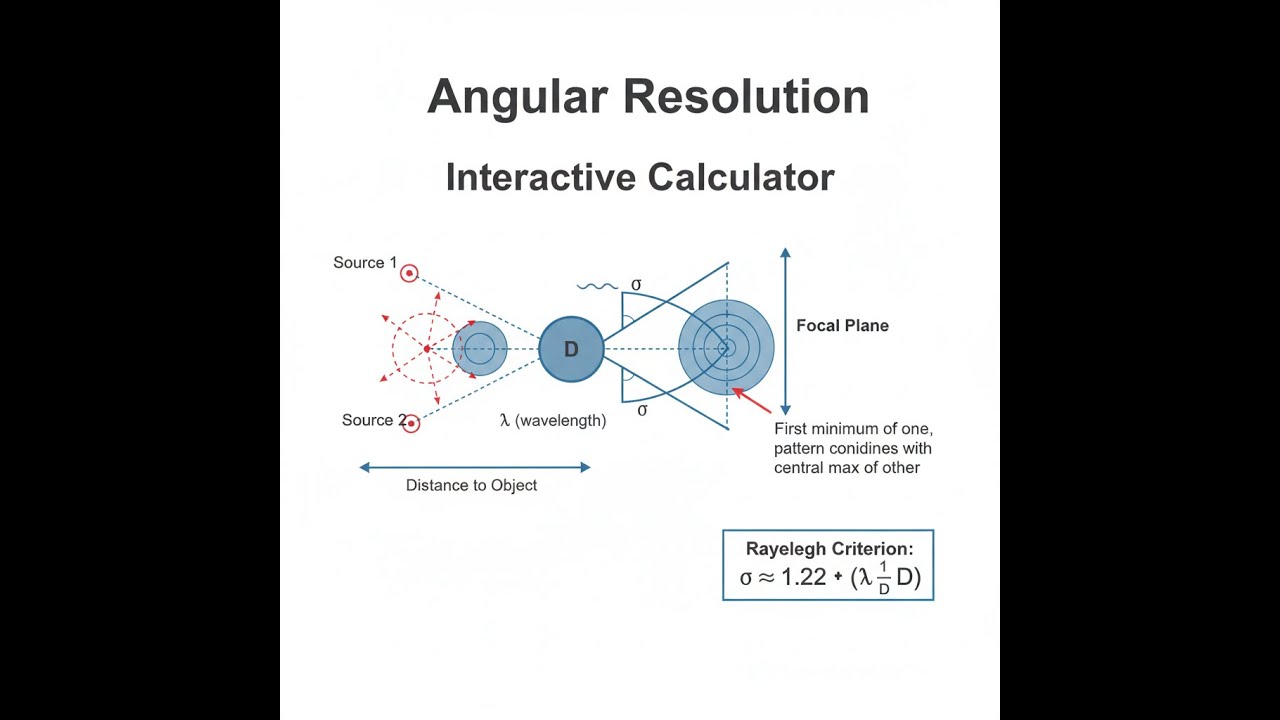
Optical System Diagram

Angular Resolution Calculator

Key Equations

Theory & Practical Applications

Physical Origin of Diffraction-Limited Resolution

Angular resolution in optical systems is fundamentally limited by the wave nature of light. When light passes through a circular aperture, diffraction causes each point source to produce not a point image but an Airy pattern — a bright central disk surrounded by progressively dimmer concentric rings. The Rayleigh criterion defines resolution as the angular separation at which the central maximum of one Airy disk falls on the first minimum of another. At this separation, the combined intensity pattern shows a 26.5% dip between the two peaks, which human observers can just perceive as two distinct sources rather than one elongated blob.

The factor 1.22 in the Rayleigh formula arises from the first zero of the Bessel function J₁(x), which describes the radial intensity distribution of the Airy pattern. This is the mathematical consequence of Fraunhofer diffraction through a circular aperture. For non-circular apertures, different diffraction patterns emerge: rectangular apertures produce sinc-function patterns, while annular apertures (like Cassegrain telescopes with central obstructions) generate modified Airy patterns with redistributed energy in the rings. The core principle remains unchanged — smaller apertures or longer wavelengths reduce resolving power.

An often-overlooked nuance: the Rayleigh criterion assumes equal-intensity point sources and incoherent illumination. For sources of vastly different brightness, the fainter source's Airy pattern is swamped by the wings of the brighter source, requiring angular separations several times the Rayleigh limit for detection. This matters in exoplanet detection, where planets are 10⁶ to 10⁹ times dimmer than their host stars. Coronagraphs and adaptive optics address this by suppressing starlight, but the fundamental diffraction limit still determines the inner working angle of these instruments.

Atmospheric Effects and Ground-Based Astronomy

Ground-based telescopes face an additional limitation beyond diffraction: atmospheric turbulence. Temperature gradients create refractive index variations that distort incoming wavefronts on timescales of milliseconds. This "seeing" typically limits optical telescopes to ~0.5-2.0 arcsecond resolution regardless of aperture size. The Fried parameter r₀ quantifies atmospheric coherence length — effectively the aperture size over which wavefronts remain coherent. At visible wavelengths, r₀ is typically 10-20 cm at good observing sites, meaning that even a 10-meter telescope without adaptive optics performs optically like a 10-20 cm telescope.

Adaptive optics systems measure wavefront distortions using a guide star (natural or laser-generated) and compensate in real-time using deformable mirrors with hundreds or thousands of actuators. Modern AO systems achieve Strehl ratios (fraction of diffraction-limited peak intensity) of 0.4-0.8 in near-infrared, approaching theoretical resolution for large apertures. However, AO correction is wavelength-dependent (r₀ scales as λ^6/5) and limited to small fields of view, making it most effective for near-infrared imaging of compact targets.

Satellite and Reconnaissance Imaging

Spy satellites operate in the visible spectrum from orbits 200-1000 km above Earth. The Hubble Space Telescope's 2.4-meter aperture achieves ~0.05 arcsecond resolution at 500 nm — diffraction-limited without atmospheric interference. At a 600 km low-Earth orbit, this translates to ~15 cm ground resolution. Declassified Keyhole reconnaissance satellites are believed to have similar or slightly larger apertures, with resolution in the 10-15 cm range when pointed straight down. Oblique viewing increases the effective distance and degrades resolution according to the slant range and atmospheric path length.

The relationship between orbit altitude, aperture, and resolution drives satellite design tradeoffs. Lower orbits provide better resolution but require more frequent orbit maintenance due to atmospheric drag and reduce revisit times. Commercial imaging satellites like Worldview-3 (0.31 m resolution from 617 km orbit) use apertures around 1.1 meters. Military satellites likely push larger apertures (3-4 meters) to the edge of launch vehicle fairing constraints. Diffraction fundamentally limits resolution improvement beyond aperture scaling — no amount of computational post-processing can recover information below the diffraction limit, though super-resolution techniques can slightly improve effective resolution when imaging extended scenes with known statistical properties.

Microscopy and Numerical Aperture

Optical microscopes face the same diffraction physics but use numerical aperture (NA) rather than physical diameter to characterize resolution. NA = n sin(α), where n is the refractive index of the imaging medium and α is the half-angle of the light cone entering the objective. High-NA objectives (NA = 1.4 with oil immersion, n = 1.515) collect light over larger solid angles, improving resolution. The Abbe diffraction limit d = λ/(2·NA) gives minimum resolvable distance for incoherent illumination.

At NA = 1.4 and λ = 500 nm (green light), resolution reaches ~180 nm — sufficient to resolve large cellular organelles but inadequate for molecular-scale imaging. This limitation drove development of super-resolution techniques: STED microscopy uses stimulated emission depletion to narrow the effective point spread function below the diffraction limit; PALM/STORM exploit photoswitchable fluorophores to localize individual molecules with ~20 nm precision through repeated imaging and statistical analysis. These methods circumvent rather than violate the diffraction limit by encoding additional information (temporal or spectral) that allows computational reconstruction beyond the Abbe limit.

Worked Example: Telescope Performance Analysis

Scenario: An amateur astronomer is evaluating whether a 203 mm (8-inch) Schmidt-Cassegrain telescope can resolve the Cassini Division in Saturn's rings (gap width ~4800 km) when Saturn is at opposition distance of 1.28 × 10⁹ km. Observation is at 550 nm (peak visual sensitivity), assuming near-perfect atmospheric seeing of 0.8 arcseconds and using the Dawes criterion (0.82 instead of 1.22) typical for visual double-star work.

Step 1: Calculate diffraction-limited angular resolution

Using the Dawes criterion: θ = 0.82 × λ / D

θ = 0.82 × (550 × 10⁻⁹ m) / (0.203 m)

θ = 2.223 × 10⁻⁶ radians

Converting to arcseconds: θ = 2.223 × 10⁻⁶ × (180/π) × 3600 = 0.458 arcseconds

Step 2: Calculate angular size of Cassini Division

Linear size s = 4800 km = 4.8 × 10⁶ m

Distance r = 1.28 × 10⁹ km = 1.28 × 10¹² m

Angular size θ_obj = s / r = (4.8 × 10⁶) / (1.28 × 10¹²) = 3.75 × 10⁻⁶ radians

θ_obj = 3.75 × 10⁻⁶ × (180/π) × 3600 = 0.773 arcseconds

Step 3: Compare to atmospheric seeing limit

Diffraction limit: 0.458 arcseconds

Atmospheric seeing: 0.8 arcseconds (specified)

Effective resolution: limited by seeing, ~0.8 arcseconds

Step 4: Evaluate detectability

Cassini Division angular width: 0.773 arcseconds

Effective telescope resolution: 0.8 arcseconds

Ratio: 0.773 / 0.8 = 0.97

Conclusion: The Cassini Division is marginally detectable under these conditions. The gap width (0.773 arcsec) is just slightly smaller than the effective resolution (0.8 arcsec). In practice, the observer would see the Cassini Division as a very subtle darkening rather than a clean gap. The limiting factor is atmospheric seeing, not aperture — the diffraction limit (0.458 arcsec) is 1.7× better than needed. On a night with exceptional seeing (0.5 arcsec), the Division would be clearly visible. This illustrates why experienced planetary observers prioritize observing sites with good seeing over larger apertures: a 150 mm telescope at 0.5 arcsec seeing outperforms a 300 mm telescope at 1.5 arcsec seeing for planetary detail. The calculation also shows why space-based observation (Hubble, JWST) revolutionized high-resolution astronomy — eliminating atmospheric turbulence allows full exploitation of aperture-limited resolution.

Wavelength Scaling and Multi-Spectral Systems

Resolution scales linearly with wavelength, creating significant challenges for infrared imaging systems. A 1-meter telescope achieves 0.138 arcseconds at 550 nm but only 1.38 arcseconds at 5.5 μm (mid-infrared). Radio telescopes face even starker limitations: a single 100-meter radio dish at 21 cm wavelength (neutral hydrogen line) has angular resolution of ~0.044 radians (2.5°) — effectively blind compared to optical systems. This drives radio astronomy to interferometric arrays like ALMA (Atacama Large Millimeter Array), which synthesizes apertures up to 16 km using phase-coherent combination of signals from multiple dishes. The Very Long Baseline Array achieves continent-scale baselines (8000+ km), providing microarcsecond resolution for radio imaging — far exceeding optical capabilities through fundamentally different physics.

Ultraviolet astronomy benefits from shorter wavelengths: at 150 nm, a space telescope achieves resolution 3.7× better than at visible wavelengths. However, UV optics face material challenges (absorption in glass, specialized coatings) and must operate above Earth's atmosphere. X-ray telescopes cannot use conventional refractive or reflective optics due to high photon energy; grazing-incidence mirrors at shallow angles provide focusing, with resolution limited by surface figure errors rather than diffraction. The Chandra X-ray Observatory achieves 0.5 arcsecond resolution through sub-nanometer mirror figure accuracy — a manufacturing marvel enabling spatial resolution that would require a 100-meter optical telescope.

Computational Imaging and Resolution Enhancement

While diffraction fundamentally limits information content in a single image, multi-image techniques extract additional resolution. Lucky imaging captures thousands of short-exposure frames, selecting and combining those with minimal atmospheric distortion to approach diffraction-limited resolution from ground-based telescopes. Speckle interferometry analyzes the statistical properties of rapidly-changing speckle patterns to reconstruct diffraction-limited images. Synthetic aperture radar (SAR) exploits platform motion to synthesize large effective apertures: a satellite with a 10-meter antenna can generate imagery equivalent to a 1-kilometer aperture by coherently combining radar returns over its orbital path.

Computational super-resolution algorithms like Richardson-Lucy deconvolution can partially reverse point spread function blurring, improving effective resolution by ~20-30% when the PSF is well-characterized. However, these methods amplify noise and can introduce artifacts if pushed beyond physically justified limits. Machine learning approaches trained on high-resolution ground truth can sometimes infer sub-diffraction details by recognizing statistical patterns, but this represents prediction rather than measurement — fine for standardized targets, dangerous for scientific discovery where unknown structures must be reliably detected.

Frequently Asked Questions