Throughput Littles Law Interactive Calculator

Little's Law is a fundamental theorem in queueing theory that relates the average number of items in a system, the average arrival rate, and the average time items spend in the system. This interactive calculator enables engineers, manufacturing managers, and operations analysts to optimize system performance, predict bottlenecks, and calculate throughput across production lines, service queues, and inventory systems.

Understanding the relationship between work-in-process (WIP), cycle time, and throughput is essential for lean manufacturing, capacity planning, and continuous improvement initiatives across industries from semiconductor fabrication to healthcare delivery.

📐 Browse all free engineering calculators

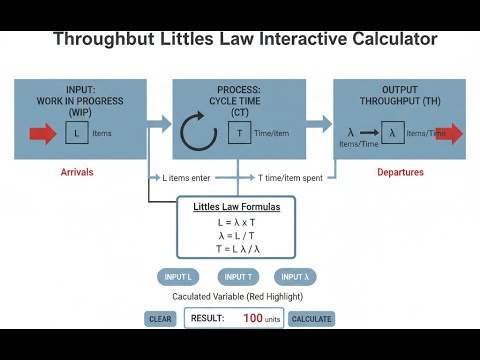
System Diagram

Interactive Throughput Calculator

Equations & Formulas

Theory & Engineering Applications

Little's Law, formulated by John Little in 1961 and rigorously proven in 1970, stands as one of the most powerful and universally applicable theorems in operations research and queueing theory. Unlike many theoretical models that require restrictive assumptions about probability distributions or system behavior, Little's Law holds true under remarkably general conditions: it requires only that the system reaches a steady state and that the average arrival rate equals the average departure rate over the long term.

Mathematical Foundation and Proof Requirements

The elegance of Little's Law lies in its simplicity and generality. The relationship L = λW does not depend on the arrival process distribution (Poisson, deterministic, or arbitrary), the service time distribution, the network topology, the service discipline (FIFO, LIFO, priority), or the number of servers. This remarkable robustness makes it applicable to manufacturing lines, computer networks, hospital emergency departments, and financial transaction systems alike.

For the law to hold rigorously, three conditions must be satisfied: (1) the system must operate in statistical equilibrium (steady state), meaning long-term arrival rate equals departure rate; (2) the observation period must be sufficiently long to average out transient effects; and (3) all items that enter the system eventually leave. The third condition is occasionally violated in practice when items can be lost, abandoned, or permanently stored, requiring careful interpretation.

One non-obvious insight concerns the time-averaging versus ensemble-averaging distinction. Little's Law relates time-averaged quantities (average number in system over time) to customer-averaged quantities (average time spent by customers). The proof relies on sample-path analysis, tracking the cumulative arrivals and departures over time. This mathematical subtlety has practical implications: measurements must be taken over appropriate time scales to capture representative behavior, particularly in systems with significant variability or cyclical patterns.

WIP, Throughput, and Cycle Time Relationships

In manufacturing and production systems, Little's Law provides the theoretical foundation for lean manufacturing principles and Theory of Constraints methodology. Work-in-Process (WIP) represents all inventory items between the start and end of a process, including raw materials being processed, items waiting in queues, and finished goods awaiting shipment. Reducing WIP without decreasing throughput necessarily reduces cycle time, which translates to faster customer delivery, reduced carrying costs, and improved cash flow.

The relationship reveals a fundamental tradeoff in system design. For a given throughput requirement, cycle time and WIP are directly proportional. Reducing cycle time requires either reducing WIP (which may risk throughput if variability is high) or increasing throughput capacity. Conversely, capacity-constrained systems often accumulate WIP as buffers against variability, but this increases cycle time predictably according to Little's Law.

A critical practical limitation emerges in highly variable systems. While Little's Law provides the average relationship, it says nothing about variance or higher-order moments. A system with average WIP of 50 items and average cycle time of 5 hours has average throughput of 10 items/hour, but individual items might experience cycle times ranging from 2 to 20 hours depending on variability in arrival times and processing rates. Queueing theory extensions like Kingman's formula are required to predict these variances.

Manufacturing and Production Line Applications

In semiconductor fabrication, where cycle times can span weeks or months and WIP values in the thousands, Little's Law enables capacity planning and bottleneck analysis. Fabs track "X-factor" (actual cycle time divided by theoretical minimum cycle time) as a key performance metric. By applying Little's Law to individual process steps, engineers can identify where WIP accumulates and cycle time extends beyond theoretical minimums, revealing hidden bottlenecks and inefficiencies.

Automotive assembly lines use Little's Law to balance production rates across workstations. If Station A produces 60 vehicles/hour with average WIP of 15 vehicles, its cycle time is 0.25 hours (15 minutes). If downstream Station B has WIP of 30 vehicles with the same throughput requirement, its cycle time must be 0.5 hours (30 minutes), indicating either slower processing or higher variability requiring additional buffer inventory. This analysis guides continuous improvement efforts and capital investment decisions.

For more complex applications, explore our complete collection of engineering calculators covering production planning, inventory optimization, and system dynamics.

Service Systems and Healthcare Applications

Emergency departments apply Little's Law to manage patient flow and reduce overcrowding. If an ED sees 120 patients per day (5 patients/hour) and average length of stay is 4.2 hours, the expected number of patients in the department at any time is 21 patients. This prediction helps determine staffing requirements, bed capacity, and triage protocols. Deviations from predicted values signal process breakdowns requiring intervention.

Call centers use the relationship to size agent pools and predict wait times. With 300 calls/hour arriving and average call duration of 6 minutes (0.1 hours), steady-state operation requires at least 30 agents (300 × 0.1). Adding queue wait time to handle variability, total cycle time might be 8 minutes, predicting 40 customers in the system on average (300 × 0.133). Service level agreements and customer satisfaction targets drive the balance between staffing costs and acceptable wait times.

Software Development and Agile Methodology

Agile teams apply Little's Law under the name "Cumulative Flow Diagram" analysis. If a development team has 24 stories in progress (WIP) and completes 8 stories per week (throughput), average cycle time is 3 weeks. To reduce cycle time to 2 weeks without changing team capacity, WIP must decrease to 16 stories. This drives work-in-progress limits in Kanban systems and sprint planning in Scrum methodologies.

The law reveals why multitasking degrades performance. An engineer working on 5 concurrent projects with 8 hours/day available (throughput of 0.2 projects/day assuming 40-hour projects) will have average cycle time of 25 days per project (5 ÷ 0.2). Reducing WIP to 2 concurrent projects cuts cycle time to 10 days, delivering customer value faster despite unchanged individual productivity.

Worked Example: PCB Assembly Line Optimization

A printed circuit board assembly facility operates a surface-mount technology (SMT) line producing automotive control modules. Current performance metrics show:

• Average WIP: 187 boards on the line
• Average throughput: 23.4 boards/hour measured over two weeks
• Theoretical minimum processing time: 4.2 minutes/board (all stations operating continuously)
• Production operates 18 hours/day, 6 days/week

Step 1: Calculate Current Cycle Time

Applying Little's Law: CT = WIP / TH

CT = 187 boards ÷ 23.4 boards/hour = 7.991 hours

Current cycle time is approximately 8.0 hours per board.

Step 2: Calculate Theoretical Minimum Cycle Time

Theoretical CT_min = 4.2 minutes = 0.070 hours

This represents pure processing time with zero queue time or delays.

Step 3: Calculate X-Factor (Efficiency Metric)

X-Factor = Actual CT / Theoretical CT = 7.991 hours ÷ 0.070 hours = 114.2

The actual cycle time is 114 times the theoretical minimum, indicating substantial opportunity for improvement. Industry best practice for well-managed SMT lines is X-Factor between 3 and 10.

Step 4: Decompose Cycle Time into Components

Processing time per board: PT = 1 / TH = 1 ÷ 23.4 = 0.0427 hours (2.56 minutes)

Wait time per board: WT = CT - PT = 7.991 - 0.0427 = 7.948 hours

Wait time percentage: (7.948 ÷ 7.991) × 100% = 99.5%

Boards spend 99.5% of cycle time waiting rather than being actively processed, revealing massive inefficiency.

Step 5: Calculate Capacity Under Optimal Conditions

If WIP were reduced to optimal level with minimal wait time, assume achievable CT = 0.5 hours (30 minutes, representing X-Factor of 7.1):

Required WIP for current throughput: WIP = TH × CT = 23.4 × 0.5 = 11.7 boards

Alternatively, maintaining current WIP but improving flow:

Maximum throughput: TH_max = WIP / CT_min = 187 ÷ 0.070 = 2,671 boards/hour (theoretical ceiling)

Realistic maximum (assuming X-Factor of 5): TH_realistic = 187 ÷ (0.070 × 5) = 534 boards/hour

Current utilization: U = 23.4 ÷ 534 = 4.4% of realistic capacity

Step 6: Develop Improvement Recommendations

Target state: Reduce WIP to 25 boards (87% reduction) while maintaining 23.4 boards/hour throughput

Target cycle time: CT_target = 25 ÷ 23.4 = 1.07 hours (64 minutes)

This represents an 86.6% cycle time reduction, improving delivery speed and reducing inventory carrying costs by $X per day (depending on board value and cost of capital).

To achieve this requires identifying and eliminating the root causes of excessive wait time: machine downtime, changeover delays, material shortages, batch processing instead of single-piece flow, and quality defects requiring rework.

This worked example demonstrates how Little's Law transforms abstract performance metrics into actionable improvement targets with quantified financial impact.

Practical Applications

Frequently Asked Questions