Soil Classification Uscs Interactive Calculator

Geotechnical engineers and site investigators routinely collect grain size data and Atterberg limits from lab tests — but translating those raw numbers into a defensible USCS group symbol requires navigating a branching set of criteria that's easy to get wrong. Use this Soil Classification USCS Interactive Calculator to determine your soil's group symbol, group name, and key engineering properties using grain size percentages, gradation coefficients, liquid limit, and plasticity index. It matters across foundation design, earthwork specification, pavement subgrade evaluation, and site investigation reporting. This page includes the full USCS classification criteria, worked examples, theory behind the plasticity chart and gradation coefficients, and a detailed FAQ.

What is USCS Soil Classification?

USCS — the Unified Soil Classification System — is a standardized method for sorting soils into engineering behavior groups based on particle size and plasticity. Give it your lab test data and it returns a 2-letter symbol (like GW, CL, or OH) that tells you how that soil will perform under load, drainage, and compaction.

Simple Explanation

Think of USCS as a sorting system for dirt. It asks two basic questions: how big are the particles, and how sticky is the soil when wet? A coarse, gravelly soil with no clay gets a different label — and very different design rules — than a fine, plastic clay. The label you end up with is shorthand for a whole set of engineering expectations: how strong it is, how well it drains, how much it compresses.

📐 Browse all 1000+ Interactive Calculators

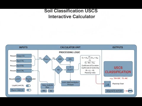
Visual Diagram

Interactive USCS Soil Classification Calculator

How to Use This Calculator

1. Select your classification mode from the dropdown — Coarse-Grained, Fine-Grained, Gradation Analysis, Plasticity Classification, or Organic Content Assessment — depending on what lab data you have.
2. Enter your grain size percentages (gravel, sand, fines), gradation coefficients (C_u, C_c), or Atterberg limits (LL, PL, PI) in the visible input fields for your selected mode.
3. Check that percentages sum to approximately 100% and that all required fields for your mode are filled in.
4. Click Calculate to see your result.

Simple Example

You have a soil with 60% fines passing the No. 200 sieve, a liquid limit of 52%, and a plasticity index of 24%. Select Fine-Grained mode, enter those 3 values, and click Classify Soil. Result: CH — Fat clay. High plasticity, very low permeability, very high compressibility. Deep foundations or ground improvement required.

Classification Criteria & Equations

Theory & Engineering Applications

The Unified Soil Classification System represents one of the most significant standardizations in geotechnical engineering history. Developed by Arthur Casagrande during World War II for military airfield construction and later refined by the U.S. Army Corps of Engineers, the USCS correlates observable soil properties with engineering behavior more effectively than any predecessor system. The genius of USCS lies in its dual-parameter approach: coarse-grained soils are classified by grain size distribution and gradation geometry, while fine-grained soils are classified by plasticity characteristics that directly relate to clay mineralogy and particle surface activity.

Coarse-Grained Soil Classification

When more than 50% of soil mass is retained on the No. 200 sieve (0.075 mm opening), the material exhibits granular behavior dominated by interparticle friction rather than cohesion. The primary subdivision distinguishes gravel (G) from sand (S) based on whether the coarse fraction is predominantly retained on (gravel) or passes through (sand) the No. 4 sieve (4.75 mm). This threshold reflects a critical behavioral transition: gravels develop higher internal friction angles (typically 38-45°) compared to sands (30-38°), and exhibit superior drainage characteristics that make them preferred materials for drainage layers and free-draining fills.

The secondary classification of coarse soils depends critically on fines content. For clean sands and gravels (less than 5% passing No. 200), gradation geometry determines the classification as well-graded (W) or poorly-graded (P). The coefficient of uniformity (C_u) quantifies the range of particle sizes present: higher C_u values indicate better gradation with sizes spanning multiple orders of magnitude. The coefficient of curvature (C_c) measures the shape of the grain size distribution curve, identifying gap-graded soils (missing middle sizes) that behave poorly despite high C_u values. Well-graded materials achieve superior compaction density, higher shear strength, and lower permeability compared to uniform or gap-graded soils because smaller particles fill voids between larger grains, creating a denser particle matrix. This explains why well-graded gravels serve as optimal base courses for pavements and railroad ballast.

When fines content reaches 5-12%, the soil receives a dual classification (e.g., SW-SC) acknowledging that both gradation and plasticity influence behavior. Above 12% fines, the matrix of fine particles controls engineering properties, and classification shifts entirely to plasticity-based symbols (SM, SC, GM, GC). This transition reflects a fundamental mechanical shift: coarse particles create the load-bearing skeleton below 12% fines, but above this threshold, fine particle interactions dominate consolidation, permeability, and shear behavior.

A critical practical consideration emerges here — many specification writers incorrectly assume all SM or SC soils behave similarly, when in fact SM materials with 13% fines differ dramatically from those with 45% fines in compaction response, strength gain, and moisture sensitivity.

Fine-Grained Soil Classification and the Plasticity Chart

Fine-grained soils derive their engineering behavior from particle surface forces, clay mineralogy, and water adsorption rather than grain-to-grain contact. The Casagrande plasticity chart — plotting liquid limit versus plasticity index — brilliantly correlates these parameters with fundamental soil behavior. The A-line (PI = 0.73(LL-20)) represents an empirical boundary separating clay-like behavior (above the line) from silt-like behavior (below the line). This distinction matters profoundly: clays exhibit true plasticity with their range of moldable consistency, while silts behave more like very fine sands, showing limited plasticity and rapid strength loss when disturbed.

The 50% liquid limit threshold dividing low (L) from high (H) plasticity reflects clay mineralogy differences. Low-plasticity clays (CL) typically contain kaolinite or illite minerals with limited surface activity, yielding moderate shrink-swell potential and consolidation rates of 1-10 years for typical foundation loading. High-plasticity clays (CH), often containing montmorillonite or smectite minerals, exhibit extreme shrink-swell behavior (volume changes exceeding 10%), very slow consolidation (decades for thick deposits), and dramatically reduced shear strength when remolded. The classification of a soil as CH rather than CL immediately signals the need for deep foundations, moisture-control measures, and careful attention to post-construction settlement.

Elastic silts (MH) represent a particularly troublesome classification. Despite plotting in the high-plasticity region, these materials — often micaceous silts, diatomaceous earth, or volcanic soils — exhibit extreme sensitivity to disturbance, very high compressibility, and poor strength characteristics. The "elastic" designation comes from their behavior when squeezing a wet sample: it rebounds slightly when pressure releases, unlike clay which remains deformed. Many foundation failures occur when MH soils are mistakenly treated as high-strength materials based solely on their high liquid limit, when in fact they require ground improvement or deep foundations similar to organic soils.

Organic Soil Identification

Organic soils present special challenges because organic matter dramatically alters plasticity behavior while contributing essentially zero strength. The USCS employs the oven-drying test to detect organic influence: if the liquid limit drops by more than 25% after oven-drying (indicating LL_dried/LL_not-dried less than 0.75), organic material is present in sufficient quantity to warrant an O designation (OL or OH). This test works because organic compounds decompose or oxidize during oven-drying, removing their contribution to water retention. Alternatively, organic content can be quantified directly through loss-on-ignition testing, where soil is combusted at 440°C and weight loss measured — anything above 8-10% organic content typically produces observable behavioral changes.

Peat (Pt) represents the extreme end of organic soil classification, with fibrous plant material constituting the bulk of the soil mass. Peat exhibits compression ratios (strain under load) often exceeding 0.5, meaning a 1-meter-thick peat layer can compress by over 50 cm under typical structural loads. Additionally, peat decomposition continues after construction, producing long-term settlement that can persist for decades. Standard practice for construction over peat involves complete excavation and replacement, surcharging with temporary fill to pre-compress the peat before construction, or use of deep foundations that bypass the peat layer entirely. The misidentification of highly organic soil as inorganic ML or CL has caused numerous structural failures where foundations settled far beyond design predictions.

Worked Example: Complete USCS Classification

A soil sample from a proposed building site yields the following laboratory test results:

• Grain size analysis: 32.4% retained on No. 4 sieve (4.75mm), 41.7% passing No. 4 and retained on No. 200 (0.075mm), 25.9% passing No. 200 sieve
• From grain size curve: D₁₀ = 0.08 mm, D₃₀ = 0.65 mm, D₆₀ = 3.2 mm
• Atterberg limits on minus No. 40 fraction: LL = 32%, PL = 18%
• Visual observation: brown color, no organic odor

Step 1: Determine coarse vs. fine classification

Total coarse fraction = 32.4% + 41.7% = 74.1% retained on No. 200 sieve

Since 74.1% > 50%, this is a coarse-grained soil.

Step 2: Determine gravel vs. sand

Of the coarse fraction (74.1%), the percentage retained on No. 4 is: (32.4/74.1) × 100 = 43.7%

The percentage passing No. 4 is: (41.7/74.1) × 100 = 56.3%

Since more than 50% of the coarse fraction passes the No. 4 sieve, the primary classification is Sand (S).

Step 3: Evaluate fines content influence

Fines content = 25.9%, which exceeds 12%

Therefore, classification will be based on plasticity of fines (SM or SC)

Step 4: Calculate plasticity parameters

PI = LL - PL = 32 - 18 = 14%

A-line value at LL = 32: PI_A-line = 0.73(32 - 20) = 0.73 × 12 = 8.76%

Step 5: Classify fines type

Since PI = 14% > 7% AND PI = 14% > PI_A-line = 8.76%, the fines plot above the A-line and are clayey.

Step 6: Calculate gradation coefficients (for complete characterization)

C_u = D₆₀/D₁₀ = 3.2/0.08 = 40

C_c = (D₃₀)²/(D₁₀ × D₆₀) = (0.65)²/(0.08 × 3.2) = 0.4225/0.256 = 1.65

For well-graded sand: C_u ≥ 6 AND 1 ≤ C_c ≤ 3

This soil meets both criteria (40 ≥ 6, and 1.65 is between 1 and 3), so the gradation is excellent.

Final Classification: SC (Clayey Sand)

Group Name: Clayey sand, well-graded

Engineering Implications:

This SC classification with well-graded characteristics indicates a soil with favorable engineering properties. The 26% clay content provides some cohesion and reduces permeability (estimated 10^-5 to 10^-6 cm/s), while the well-graded sand skeleton provides good shear strength (friction angle approximately 32-36°) and reasonable bearing capacity (allowable bearing pressure approximately 150-250 kPa for shallow foundations). The clay binder makes this material moisture-sensitive during construction — optimum moisture content for compaction will be critical (likely 10-14%), and achieving specified density will require careful moisture control. The material should compact well to 95% Standard Proctor density with proper moisture and effort. Moderate frost susceptibility exists due to the silt-size fraction implied by the D₁₀ value of 0.08 mm (on the silt-sand boundary). For pavement subgrade applications, a frost-depth analysis would be warranted in cold climates.

Limitations and Special Considerations

While USCS provides excellent correlation with soil behavior, several limitations deserve recognition. The system classifies soils based on disturbed samples, yet many fine-grained soils exhibit dramatically different behavior in their natural, undisturbed state due to structure and cementation. A soft, sensitive marine clay may classify identically to a stiff, overconsolidated glacial clay, yet these materials require entirely different foundation approaches. The USCS symbol communicates nothing about soil sensitivity, overconsolidation ratio, natural water content relative to liquid limit, or in-situ density — all critical parameters for design.

Furthermore, the system struggles with borderline cases. Soils plotting near the A-line may receive different classifications from different laboratories due to normal testing variability in Atterberg limits (±2-3% is common). The 12% fines threshold for dual symbols creates discontinuities where soils at 11.8% and 12.2% fines receive fundamentally different symbols despite nearly identical behavior. Modern practice increasingly supplements USCS classifications with quantitative engineering parameters — consolidation coefficients, shear strength measurements, and permeability data — rather than relying solely on the classification symbol for design decisions.

For additional geotechnical engineering resources and calculation tools, visit the engineering calculator library.

Practical Applications

Frequently Asked Questions