Designing a fiber optic link means accounting for every decibel — fiber loss, connector loss, splice loss — before you commit to transceivers, amplifiers, or route distance. Use this Optical Fiber Attenuation Calculator to calculate total signal power loss through fiber optic cables using fiber length, attenuation coefficient, connector count, and splice count. Getting this right matters in telecommunications infrastructure, data center interconnects, and submarine cable systems where an undersized power budget means a failed link. This page includes the full attenuation formula, a worked example, engineering theory, and an FAQ.
What is optical fiber attenuation?
Optical fiber attenuation is the reduction in light signal strength as it travels through a fiber optic cable. It is measured in decibels (dB) and tells you how much power you lose over a given distance or through connectors and splices.
Simple Explanation
Think of it like water flowing through a long hose — the further it travels, the weaker the flow gets at the other end. In a fiber optic cable, light behaves the same way: every kilometer of fiber, every connector, and every splice takes a small bite out of the signal. Add those losses up, and that's your total attenuation.
📐 Browse all 1000+ Interactive Calculators
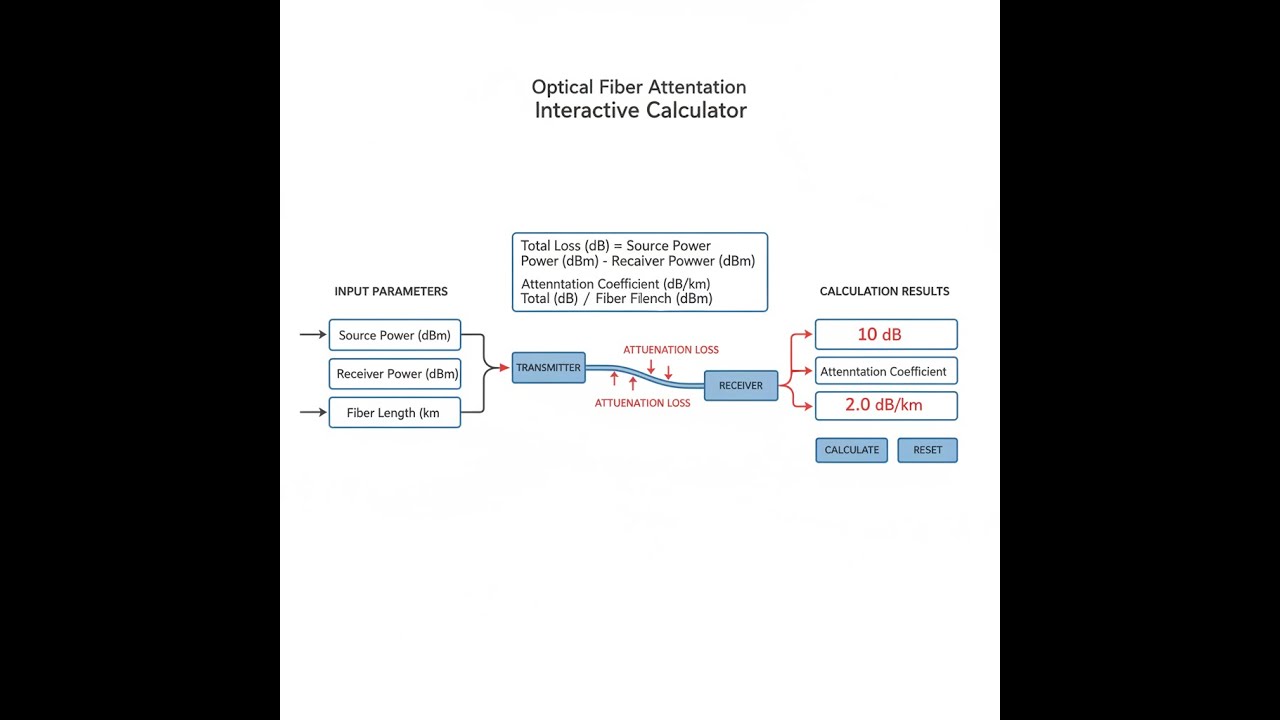
Fiber Attenuation Diagram

Optical Fiber Attenuation Calculator
How to Use This Calculator
- Select your calculation mode from the dropdown — total loss, output power, max length, or others.
- Enter your fiber length (km), attenuation coefficient (dB/km), number of connectors, and number of splices with their respective loss values.
- Adjust input or output power values as required by your selected mode.
- Click Calculate to see your result.
Optical Fiber Attenuation Interactive Visualizer
Watch how signal power drops through fiber length, connectors, and splices. Adjust parameters to see real-time attenuation calculations for fiber optic link design.
TOTAL ATTENUATION
6.05 dB
OUTPUT POWER
-6.05 dBm
LINK MARGIN
23.95 dB
FIRGELLI Automations — Interactive Engineering Calculators
Attenuation Equations
Use the formula below to calculate total fiber attenuation.
Total Fiber Attenuation
Atotal = α × L + Nc × Ac + Ns × As
Where:
Atotal = Total attenuation (dB)
α = Attenuation coefficient (dB/km)
L = Fiber length (km)
Nc = Number of connectors
Ac = Loss per connector (dB)
Ns = Number of splices
As = Loss per splice (dB)
Use the formula below to calculate output power.
Output Power Calculation
Pout = Pin - Atotal
Where:
Pout = Output power (dBm)
Pin = Input power (dBm)
Atotal = Total attenuation (dB)
Use the formula below to calculate maximum fiber length.
Maximum Fiber Length
Lmax = (Pbudget - Nc × Ac - Ns × As) / α
Where:
Lmax = Maximum fiber length (km)
Pbudget = Available power budget (dB)
α = Attenuation coefficient (dB/km)
Use the formula below to calculate link margin.
Link Margin
M = Pout - Pmin
Where:
M = Link margin (dB)
Pout = Output power at receiver (dBm)
Pmin = Minimum receiver sensitivity (dBm, typically -30 dBm)
Simple Example
Inputs: fiber length = 10 km, attenuation coefficient = 0.35 dB/km, 2 connectors at 0.5 dB each, 3 splices at 0.1 dB each, input power = 0 dBm.
Fiber loss = 0.35 × 10 = 3.5 dB. Connector loss = 2 × 0.5 = 1.0 dB. Splice loss = 3 × 0.1 = 0.3 dB.
Total attenuation = 3.5 + 1.0 + 0.3 = 4.8 dB. Output power = 0 − 4.8 = −4.8 dBm.
Theory & Engineering Applications
Optical fiber attenuation represents the fundamental limitation of fiber optic communication systems, quantifying the progressive loss of optical power as light propagates through the fiber medium. Understanding attenuation mechanisms is critical for network design, as it directly determines maximum transmission distances, required amplifier spacing, and overall system performance in telecommunications, data centers, submarine cable systems, and sensing applications.
Physical Mechanisms of Fiber Attenuation
Attenuation in optical fibers arises from two primary mechanisms: absorption and scattering. Intrinsic absorption occurs when photons interact with silicon-oxygen bonds in the glass matrix, with peak absorption wavelengths corresponding to molecular resonances. Extrinsic absorption results from impurities, particularly hydroxyl (OH⁻) ions that create absorption peaks near 1383 nm. Modern manufacturing processes have reduced OH⁻ contamination to parts-per-billion levels, enabling "low water peak" fibers with continuous low-loss transmission from 1260 nm to 1625 nm.
Rayleigh scattering, caused by microscopic density fluctuations frozen into the glass during manufacturing, represents the fundamental limit of fiber attenuation and varies inversely with the fourth power of wavelength (λ⁻⁴). This wavelength dependence explains why longer wavelengths (1550 nm) exhibit lower attenuation than shorter wavelengths (850 nm). At 850 nm, typical multimode fiber attenuation reaches 2.5 dB/km, while at 1310 nm it drops to 0.35 dB/km, and at 1550 nm achieves the theoretical minimum near 0.20 dB/km for standard single-mode fiber.
Connector and Splice Losses
Beyond intrinsic fiber attenuation, practical optical links suffer additional losses at connection points. Connector losses arise from core misalignment, air gap variations, angular misalignment, and Fresnel reflections at glass-air interfaces. High-quality physical contact (PC) connectors achieve typical insertion losses of 0.3-0.5 dB, while angle-polished connectors (APC) reduce back-reflections to below -60 dB at the cost of slightly higher insertion loss (0.5-0.8 dB).
Fusion splices, created by arc-welding fiber ends together, typically introduce only 0.05-0.1 dB loss when executed properly with automated fusion splicers. Mechanical splices, using index-matching gel and precision alignment sleeves, exhibit higher losses of 0.1-0.3 dB but offer field-deployable solutions without specialized equipment. In long-haul systems spanning hundreds of kilometers, the cumulative effect of connector and splice losses can exceed fiber attenuation, making connection point minimization a critical design consideration.
Wavelength-Dependent Attenuation and Spectral Windows
The telecommunications industry standardized specific wavelength windows based on attenuation characteristics and component availability. The O-band (1260-1360 nm) exhibits zero chromatic dispersion in standard single-mode fiber but higher attenuation. The C-band (1530-1565 nm) offers minimum attenuation and supports erbium-doped fiber amplifiers (EDFAs), making it the primary band for long-haul transmission. The L-band (1565-1625 nm) extends EDFA operation for increased capacity.
A non-obvious consideration often overlooked in link budget calculations is attenuation variation with temperature. Fiber attenuation increases approximately 0.001 dB/km per °C above 20°C due to increased Rayleigh scattering and stress-induced birefringence. In cables exposed to extreme temperature swings (-40°C to +70°C), this can add 0.1 dB/km variation, requiring appropriate margin allocation in critical systems.
Worked Example: Data Center Interconnect Link Budget
Consider designing a 15.7 km metropolitan fiber link connecting two data centers using 1310 nm single-mode fiber transceivers. The system specifications include: transceiver output power +2 dBm, receiver sensitivity -18 dBm, desired link margin 3 dB. The physical implementation requires 6 LC/UPC connectors (3 mated pairs) and 2 fusion splices at cable junction points.
Step 1: Calculate Available Power Budget
Power Budget = PTX - PRX,min - Margin
Power Budget = (+2 dBm) - (-18 dBm) - (3 dB) = 17 dB
Step 2: Calculate Connector Losses
Using LC/UPC connectors with typical 0.4 dB insertion loss:
Total Connector Loss = 6 connectors × 0.4 dB/connector = 2.4 dB
Step 3: Calculate Splice Losses
Using fusion splices with 0.08 dB typical loss:
Total Splice Loss = 2 splices × 0.08 dB/splice = 0.16 dB
Step 4: Calculate Available Budget for Fiber Attenuation
Fiber Budget = Total Budget - Connector Loss - Splice Loss
Fiber Budget = 17 dB - 2.4 dB - 0.16 dB = 14.44 dB
Step 5: Calculate Required Fiber Attenuation Coefficient
α = Fiber Budget / Length = 14.44 dB / 15.7 km = 0.92 dB/km
This calculated attenuation coefficient of 0.92 dB/km significantly exceeds the 0.35 dB/km specification for 1310 nm single-mode fiber, confirming link viability with substantial margin. The actual fiber loss would be:
Actual Fiber Loss = 0.35 dB/km × 15.7 km = 5.50 dB
Step 6: Verify Total Link Loss and Margin
Total Loss = Fiber Loss + Connector Loss + Splice Loss
Total Loss = 5.50 dB + 2.4 dB + 0.16 dB = 8.06 dB
Received Power = PTX - Total Loss = +2 dBm - 8.06 dB = -6.06 dBm
Actual Link Margin = PRX - PRX,min = -6.06 dBm - (-18 dBm) = 11.94 dB
The link exhibits 11.94 dB margin, far exceeding the 3 dB design target. This excess margin accommodates component aging (transceivers degrade ~1 dB over 20 years), repair splices, fiber bends, and temperature-induced variations. For cost optimization, designers could substitute lower-power transceivers or extend the link distance while maintaining adequate margin.
Nonlinear Effects and High-Power Limitations
While linear attenuation dominates most fiber optic systems, high-power transmission introduces nonlinear effects that effectively increase signal degradation. Stimulated Raman scattering (SRS) transfers power from shorter to longer wavelengths when optical power density exceeds threshold levels around +10 dBm in single-mode fiber. Stimulated Brillouin scattering (SBS) creates backward-propagating light through acoustic wave interactions, limiting single-frequency laser power to approximately +6 dBm.
Dense wavelength-division multiplexing (DWDM) systems must also contend with four-wave mixing (FWM), where multiple wavelengths interact to create spurious signals at new frequencies. FWM intensity increases with channel power and decreases with chromatic dispersion and channel spacing. These nonlinear effects establish practical upper limits on launch power independent of receiver sensitivity, constraining link budget optimization strategies.
Amplifier Spacing and Regeneration Requirements
Long-haul fiber systems spanning thousands of kilometers require periodic signal amplification or regeneration. Erbium-doped fiber amplifiers (EDFAs) provide transparent optical amplification in the C-band with typical gain of 20-30 dB and noise figures around 4-6 dB. Amplifier spacing depends on fiber attenuation, span loss budget, and accumulated noise considerations. For 0.20 dB/km fiber at 1550 nm, typical amplifier spacing reaches 80-100 km before optical signal-to-noise ratio (OSNR) degradation limits system performance.
Submarine cable systems, representing the ultimate expression of fiber attenuation engineering, employ specialized low-loss fibers with attenuation below 0.16 dB/km and repeater spacing approaching 100 km. These systems accumulate amplified spontaneous emission (ASE) noise at each amplification stage, requiring careful OSNR management across spans exceeding 10,000 km. The relationship between attenuation, amplifier noise, and maximum transmission distance ultimately determines the feasibility and economics of transoceanic fiber routes.
For detailed fiber optic calculations and other engineering tools, visit the engineering calculator library.
Practical Applications
Scenario: Telecommunications Network Expansion
Marcus, a network planning engineer at a regional telecommunications provider, needs to validate whether existing fiber infrastructure can support new 100G coherent transmission equipment between two central offices separated by 73.2 km. Using the attenuation calculator with measured values from OTDR testing (0.22 dB/km fiber loss, 8 connectors at 0.45 dB each, 3 fusion splices at 0.06 dB each), he calculates total link loss of 19.80 dB. Comparing this against the transceiver's 28 dB power budget with required 4 dB margin, Marcus confirms the link remains viable without requiring additional amplification, saving his company approximately $85,000 in equipment costs and six weeks of installation time. The calculator's link margin display immediately highlighted that the system would operate with 4.2 dB excess margin, providing confidence for future network growth.
Scenario: Data Center Migration Planning
Jennifer, a data center architect planning a cloud provider's new availability zone, must determine the maximum distance between redundant facilities while maintaining 10G optical connectivity using existing transceiver inventory. Her transceivers provide +1 dBm output power with -14 dBm receiver sensitivity, and she requires conservative 5 dB link margin for long-term reliability. Using the maximum length calculation mode with estimated 10 connectors (0.5 dB each) and 4 splices (0.1 dB each), the calculator determines maximum viable fiber distance of 49.3 km using standard 0.35 dB/km fiber at 1310 nm. This constraint directly influences her facility site selection, eliminating three candidate locations that would have required 55+ km fiber runs and steering the project toward a viable site 42 km from the primary data center, ensuring both geographic diversity for disaster recovery and optical link feasibility within existing power budgets.
Scenario: Field Troubleshooting Degraded Link
David, a fiber optic field technician, responds to customer reports of intermittent packet loss on a 28 km campus fiber link connecting research buildings. His optical power meter measures -16.2 dBm at the receiver, while system documentation indicates the transmitter outputs +3 dBm and the receiver requires minimum -18 dBm for error-free operation. Using the attenuation coefficient calculation mode with total measured loss of 19.2 dB, known 6 connectors (0.4 dB specification), and 2 documented splices (0.1 dB specification), the calculator reveals an effective fiber attenuation of 0.60 dB/km—significantly higher than the 0.35 dB/km specification. This discrepancy points to either degraded fiber (potentially from water ingress) or undocumented splices from previous repairs. Armed with this quantitative analysis, David uses OTDR testing to locate three unauthorized mechanical splices at 1.2 dB total loss, explaining the performance degradation. Replacing these mechanical splices with fusion splices restores link margin to specification, resolving the customer issue and validating the diagnostic power of systematic attenuation analysis.
Frequently Asked Questions
▼ What is the difference between attenuation and loss in fiber optics?
▼ Why do different wavelengths have different attenuation values?
▼ How much link margin should I design into fiber optic systems?
▼ Can fiber optic cables actually improve or have negative attenuation?
▼ How do I account for fiber bends and coiling in attenuation calculations?
▼ What causes attenuation to increase over time in installed fiber?
Free Engineering Calculators
Explore our complete library of free engineering and physics calculators.
Browse All Calculators →🔗 Explore More Free Engineering Calculators
About the Author
Robbie Dickson — Chief Engineer & Founder, FIRGELLI Automations
Robbie Dickson brings over two decades of engineering expertise to FIRGELLI Automations. With a distinguished career at Rolls-Royce, BMW, and Ford, he has deep expertise in mechanical systems, actuator technology, and precision engineering.
Need to implement these calculations?
Explore the precision-engineered motion control solutions used by top engineers.


