When you need color consistency—whether it’s matching LEDs from different batches, calibrating a monitor, or setting up museum lighting—you need a common set of numbers. The CIE color space is the framework almost everyone uses, because it’s the only way to describe color precisely across suppliers and industries. If you ask for “warm white” in engineering terms, the only response that’s actually comparable between vendors is CIE chromaticity coordinates. This calculator takes care of those conversions: chromaticity, tristimulus, sRGB, CCT, and dominant wavelength, based on XYZ, RGB, or wavelength inputs. You’ll find the basic equations, a detailed worked LED binning example, technical context, and a FAQ. This is practical stuff—what you use every day in the lab or on the factory floor.
What is CIE Chromaticity?
CIE chromaticity gives you two numbers (x and y) that define the color—meaning hue and saturation—without including the intensity. That’s important because in most engineering work, the color consistency matters more than how bright the source is. This method is used everywhere from LED binning to monitor production lines.
Simple Explanation
Chromaticity is like describing what red a paint is, regardless of whether the room is in daylight or dusk. You can say “warm orange” without reference to the light level. The CIE system just turns that subjective label into fixed numbers so there’s no disagreement between engineers, manufacturers, or scientists about what color is being discussed.
📐 Browse all 1000+ Interactive Calculators
Table of Contents
CIE Chromaticity Diagram

Interactive Calculator
How to Use This Calculator
This calculator is intended for education, concept evaluation, and preliminary design. Results are based on the equations and assumptions described on this page, but cannot account for every real-world load case, tolerance, material property, environmental condition, installation detail, safety factor, code, or regulatory requirement. Verify all inputs, assumptions, units, and results independently before selecting components or using the result in a real application. Safety-critical, structural, medical, lifting, transportation, or regulated applications must be reviewed by a qualified engineer.
Questions about this calculator or found an error? Message our engineering team.
- Select your calculation mode from the dropdown — choose from XYZ to chromaticity, RGB conversions, dominant wavelength, or CCT.
- Enter the required input values for your chosen mode (XYZ tristimulus values, RGB values 0–255, wavelength in nm, or xy chromaticity coordinates).
- Use the "Try Example" button to load a pre-filled set of values if you want to see a sample result first.
- Click Calculate to see your result.
CIE Color Space Chromaticity Interactive Visualizer
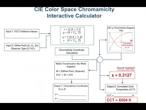
You can see directly how tweaking XYZ values shifts the chromaticity in the CIE 1931 diagram. Use the sliders and watch how the RGB value and the plotted point move—handy when troubleshooting color differences or designing for specific color bins.
x CHROMATICITY
0.410
y CHROMATICITY
0.360
CCT (K)
2856
FIRGELLI Automations — Interactive Engineering Calculators
Equations & Formulas
Use the formula below to calculate chromaticity coordinates from XYZ tristimulus values.
XYZ to Chromaticity Coordinates
x = X / (X + Y + Z)
y = Y / (X + Y + Z)
z = Z / (X + Y + Z) = 1 − x − y
Where X, Y, Z are CIE tristimulus values (dimensionless), and x, y, z are chromaticity coordinates (dimensionless, sum to unity).
Use the formula below to calculate tristimulus values from chromaticity coordinates and luminance.
Chromaticity to Tristimulus Values
X = (x / y) × Y
Z = [(1 − x − y) / y] × Y
Given chromaticity coordinates (x, y) and luminance Y, reconstruct full tristimulus values. Note: y ≠ 0 required.
Use the formula below to calculate sRGB values from XYZ tristimulus values.
XYZ to sRGB Transformation (D65)
Rlinear = 3.2405X − 1.5371Y − 0.4985Z
Glinear = −0.9693X + 1.8760Y + 0.0416Z
Blinear = 0.0556X − 0.2040Y + 1.0572Z
RsRGB = γ(Rlinear) × 255
Where γ(u) = 12.92u for u ≤ 0.0031308, else 1.055u1/2.4 − 0.055. Values clipped to [0, 255].
Use the formula below to calculate XYZ tristimulus values from sRGB inputs.
sRGB to XYZ Transformation
Rlinear = γ−1(RsRGB / 255)
X = 0.4124Rlinear + 0.3576Glinear + 0.1804Blinear
Y = 0.2127Rlinear + 0.7152Glinear + 0.0722Blinear
Z = 0.0193Rlinear + 0.1192Glinear + 0.9503Blinear
Where γ−1(u) = u/12.92 for u ≤ 0.04045, else [(u + 0.055)/1.055]2.4.
Use the formula below to calculate correlated color temperature from chromaticity coordinates.
McCamy's CCT Approximation
n = (x − 0.3320) / (0.1858 − y)
CCT = 449n³ + 3525n² + 6823.3n + 5520.33
Where CCT is correlated color temperature in Kelvin. Valid for approximately 2000 K to 10000 K near Planckian locus.
Simple Example
Given: X = 0.5, Y = 0.4, Z = 0.1 (XYZ to chromaticity mode)
Sum = 0.5 + 0.4 + 0.1 = 1.0
x = 0.5 / 1.0 = 0.500000
y = 0.4 / 1.0 = 0.400000
z = 0.1 / 1.0 = 0.100000
Theory & Engineering Applications
The CIE color spaces are the baseline for anyone trying to tie color measurements to human vision. The CIE XYZ system—going all the way back to 1931—lets you describe a color as a sum of three reference stimuli. That’s what lets you compare a display, LED, or light source with real numbers. The chromaticity diagram is just what happens when you take those three numbers and ignore how bright the light is, so you can compare color alone.
Tristimulus Values and the Fundamental Observer
XYZ values are calculated by integrating a light’s spectrum with the CIE 1931 color matching functions (x̄(λ), ȳ(λ), and z̄(λ)). In practice, this is a weighted sum over the visible range, usually 380–780 nm, with a normalization factor to match standard visual responses. Y is the only one tied to brightness perception, which makes it unique among the three. That’s why if you only care about intensity, you read off the Y.
Don’t assume this “average observer” is perfect for every application. The original CIE 1931 observer is based on data from 17 people, all with normal vision, staring at a small patch of light. If you’re designing for large fields of view or older users (whose lenses yellow), real perception will differ. Some industries use the CIE 1964 10-degree observer, and in anything high stakes—like medical imaging—you’ll run into trouble if you skip these details.
Chromaticity Coordinates: Projection to the xy Plane
Going from XYZ to chromaticity (x, y) just divides out the overall intensity, projecting the 3D color “solid” down to a flat plane. Only two values matter (x and y); z is always 1 − x − y. This 2D plot is what you see in every textbook. The curved edge is made by single-wavelength (monochromatic) lights. The straight “purple line” at the bottom connects the most extreme red and blue points—these colors don’t occur in rainbows, only by mixing red and blue light (non-spectral purples). Anything outside this shape is mathematically possible but physically unrealizable.
The white point is not fixed; it depends on what you pick for your standard illuminant. D65 simulates daylight and is used as the white for sRGB and most monitors. If you’re under tungsten (Illuminant A), the white point shifts closer to yellow/orange. Changing the white point changes how all the other colors “sit” in the space—a source of confusion if you forget to set or communicate this reference.
Color Gamut and the RGB Transformation
The sRGB triangle on the chromaticity plot is the limit for most displays. Those primary corner points were chosen to cover as much “useful” space as possible, but there are plenty of visible colors outside this triangle. The matrix for XYZ to RGB comes from matching those primary chromaticity coordinates and the white point—if you need to design a display, you’ll spend time with these matrices.
The gamma curve in sRGB isn’t a single power law. The knee near zero prevents large jumps for dark values—important to avoid visible steps at low brightness. The nonlinearity matches how our eyes respond to brightness (the Weber-Fechner law), letting us squeeze more useful color steps into 8 bits per channel than we’d get with a straight line. This is why most color encodings apply gamma correction, not just for old CRTs but for digital storage efficiency.
If you feed in XYZ data corresponding to a color outside the sRGB triangle, your calculated RGB values may go negative or above 1. The calculator clips them for practicality, but that distorts color. Professional workflows use different “gamut mapping” methods; clipping is simple but usually the worst option for visual quality.
Serious color management always works in larger spaces, applies gamut mapping, and understands the visual effects—not just the math—of the chosen transformation.
Correlated Color Temperature and the Planckian Locus
The Planckian locus is what you get if you plot where a perfect black-body radiator falls in (x, y) as its temperature is swept from red-hot to white-hot—forming a curved line across the chromaticity diagram. Correlated color temperature (CCT) just asks: for a given measured color, what temperature black-body does it most resemble? McCamy’s formula is a fast, convenient way to get CCT for most practical cases. For colors far away from the locus (highly saturated LEDs), the formula is less meaningful, and more precise calculations use iterative lookups against measured blackbody data.
It’s important to know that CCT only tells you how “warm” or “cool” a light seems for near-white sources. For a deep red or green LED, the CCT number loses meaning—it doesn’t tell you what a human perceives. And two lights with the same CCT can have completely different spectra and color rendering. Always check Duv (distance from locus) as well as CCT for real quality control.
Industrial Application: Display Calibration and Color Management
Display makers rely on chromaticity data for every unit on the production line. After assembly, they measure the panel’s white point (D65 for computer monitors), making sure chromaticity error stays within small limits—typically using CIE 1976 u'v' coordinates for this, not (x, y), because u'v' matches our ability to see color shifts. Failing to hold these tolerances results in obviously mismatched screens in a multi-monitor setup.
Color management in software depends on moving images between device color spaces (camera to monitor to printer), each with different RGB primaries and gamuts. This is handled by ICC profiles—transformation recipes, using these XYZ equations, stored with the image or the device driver. If you want consistent color across different devices, you must do these conversions at each step or accept unpredictable color shifting. Gamut mapping is crucial here—ideally using perceptual algorithms, not brute-force clipping.
Worked Example: LED Color Binning
An LED maker wants all their warm white LEDs to fall in the range 3000 K ± 150 K. They measure a batch: X = 0.3847, Y = 0.3512, Z = 0.1763. Is it within spec?
Step 1: Find the chromaticity coordinates.
Sum = 0.3847 + 0.3512 + 0.1763 = 0.9122
x = 0.3847 / 0.9122 = 0.4217
y = 0.3512 / 0.9122 = 0.3850
Step 2: Use McCamy’s formula for CCT.
n = (0.4217 − 0.3320) / (0.1858 − 0.3850) = −0.4502
Plug into the formula: CCT = 449(−0.4502)³ + 3525(−0.4502)² + 6823.3(−0.4502) + 5520.33 = 3121.9 K
Step 3: Does it pass? Yes: 3121.9 K is within [2850 K, 3150 K].
Step 4: For full QC, check distance from Plankian locus—use u'v' (not shown in all labs, but best practice for consistent results).
u' = 4X/(X + 15Y + 3Z) = 0.2490, v' = 9Y/(X + 15Y + 3Z) = 0.5115
Compare to locus at 3122 K: u'BB ≈ 0.2523, v'BB ≈ 0.5193
Duv = sqrt((−0.0033)² + (−0.0078)²) = 0.0084
This part matters: the chromaticity is just below the blackbody line, showing the familiar greenish shift seen in many white LEDs. That’s why for LED binning, CCT alone won’t guarantee visible uniformity—both CCT and Duv are needed to sort for true color consistency.
For more color and optical engineering calculations, visit our comprehensive engineering calculator library.
Practical Applications
Scenario: Display Manufacturing Quality Control
Jessica, a display engineer at an OLED panel manufacturing facility, needs to verify that the white point of a production batch meets the sRGB specification for computer monitors. Using a spectroradiometer, she measures the tristimulus values of the panel's D65 white at maximum brightness: X = 89.47, Y = 94.38, Z = 102.81. She uses the CIE chromaticity calculator to convert these values to xy coordinates, obtaining x = 0.3119, y = 0.3289. Comparing against the D65 target of (0.3127, 0.3290), she calculates the chromaticity error: Δx = 0.0008, Δy = 0.0001, well within the ±0.003 tolerance for professional displays. The batch passes QC and proceeds to final assembly, ensuring customers receive accurately calibrated monitors for color-critical work.
Scenario: Architectural Lighting Design
Marco, a lighting designer for a museum renovation, must specify LED fixtures that provide warm white illumination at 2700 K while maintaining high color rendering for artwork. The manufacturer provides specification sheets listing chromaticity coordinates (x = 0.4578, y = 0.4101) for their museum-grade LEDs. Marco uses the chromaticity to CCT calculator, which returns 2687 K—close to the target. However, he also calculates the distance from the Planckian locus in u'v' space and finds Duv = +0.0023, indicating a slightly pinkish tint above the blackbody curve. This positive Duv is acceptable for museum applications where slight warmth enhances the appearance of paintings and textiles. He specifies this LED bin for the 300+ fixtures in the gallery spaces, ensuring consistent, flattering illumination throughout the museum.
Scenario: Spectroscopy and Color Science Research
Dr. Aisha, a vision scientist studying color perception under narrow-band LED illumination, measures the spectral power distribution of a 530 nm green LED using her spectrometer. The software outputs CIE XYZ values of (0.1847, 0.6782, 0.1194) after integrating the measured spectrum with the 1931 standard observer color matching functions. To visualize where this stimulus falls on the chromaticity diagram relative to the spectral locus, she converts to xy coordinates using the calculator: x = 0.1891, y = 0.6946. Plotting this point, she confirms it lies very close to the spectral locus near 530 nm, as expected for a narrow-band LED. She then uses the dominant wavelength calculation mode to verify that observers would perceive this as 529.3 nm monochromatic light, validating her LED source for psychophysical experiments on wavelength discrimination thresholds.
Frequently Asked Questions
Free Engineering Calculators
Explore our complete library of free engineering and physics calculators.
Browse All Calculators →🔗 Explore More Free Engineering Calculators
About the Author
Robbie Dickson — Chief Engineer & Founder, FIRGELLI Automations
Robbie Dickson brings over two decades of engineering expertise to FIRGELLI Automations. With a distinguished career at Rolls-Royce, BMW, and Ford, he has deep expertise in mechanical systems, actuator technology, and precision engineering.
Video Walkthrough - How to Use This Calculator
Need to implement these calculations?
Explore the precision-engineered motion control solutions used by top engineers.


