Picking the wrong cutoff frequency — or the wrong R and C values — can ruin a sensor signal, introduce aliasing into an ADC system, or let noise straight through your power supply rail. Use this RC Filter Interactive Calculator to calculate cutoff frequency, required capacitance, required resistance, or full frequency response using resistance, capacitance, and operating frequency as inputs. It covers both low-pass and high-pass configurations across applications like audio crossover design, anti-aliasing for data acquisition, and biomedical signal conditioning. This page includes the core formulas, a worked anti-aliasing design example, plain-English theory, and a full FAQ.
What is an RC Filter?
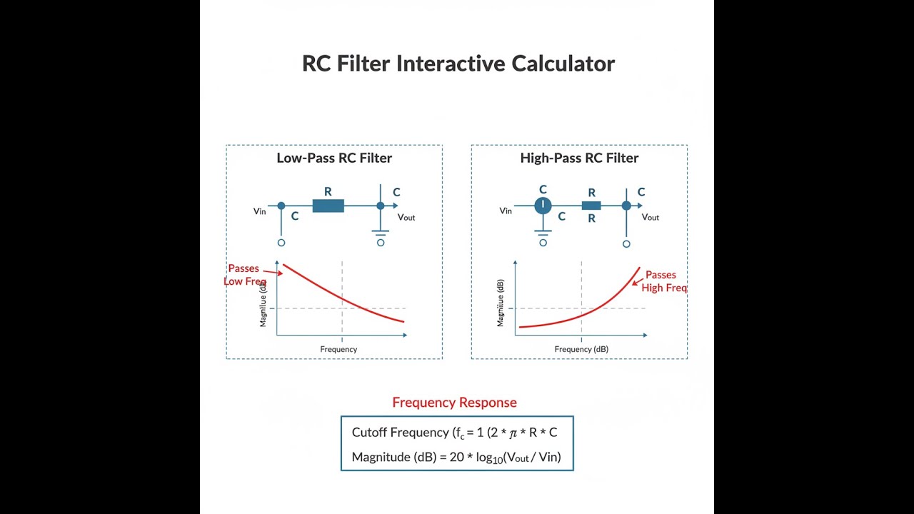
An RC filter is a simple circuit made from a resistor and a capacitor that passes some frequencies and blocks others. Depending on how you connect the two components, you get either a low-pass filter (passes low frequencies, blocks high ones) or a high-pass filter (passes high frequencies, blocks low ones).
Simple Explanation
Think of an RC filter like a gate that opens or closes depending on how fast a signal is changing. A low-pass RC filter is like a slow-moving gate — fast signals can't get through, but slow ones pass easily. The resistor and capacitor together set the speed of that gate, which is what we call the cutoff frequency.
📐 Browse all 1000+ Interactive Calculators
RC Filter Circuit Diagram

How to Use This Calculator
- Select your filter type and calculation mode from the dropdown — choose whether you want to solve for cutoff frequency, capacitance, resistance, or frequency response, and whether it's a low-pass or high-pass configuration.
- Enter your known values. Depending on the mode selected, you'll enter resistance (Ω), capacitance (F), cutoff frequency (Hz), and/or operating frequency (Hz) into the visible input fields.
- If you're unsure what values to use, click Try Example to load a working set of values for the selected mode.
- Click Calculate to see your result.
RC Filter Interactive Calculator
RC Filter Interactive Visualizer
Visualize how resistance and capacitance values affect RC filter frequency response in real-time. Watch the cutoff frequency shift as you adjust component values and see the dramatic difference between low-pass and high-pass configurations.
CUTOFF FREQ
15.9 Hz
GAIN
0.707
PHASE
-45°
FIRGELLI Automations — Interactive Engineering Calculators
RC Filter Equations
Use the formula below to calculate the cutoff frequency of an RC filter.
Cutoff Frequency
fc = 1 / (2πRC)
Where:
fc = cutoff frequency (Hz)
R = resistance (Ω)
C = capacitance (F)
π ≈ 3.14159
Angular Cutoff Frequency
ωc = 2πfc = 1 / (RC)
Where:
ωc = angular cutoff frequency (rad/s)
Time Constant
τ = RC
Where:
τ = time constant (seconds)
This represents the time for the output to reach 63.2% of its final value
Low-Pass Filter Transfer Function
H(jω) = 1 / √(1 + (ω/ωc)2)
Where:
H(jω) = voltage gain magnitude at frequency ω
ω = operating angular frequency (rad/s)
High-Pass Filter Transfer Function
H(jω) = (ω/ωc) / √(1 + (ω/ωc)2)
Where:
H(jω) = voltage gain magnitude at frequency ω
Attenuation in Decibels
AdB = 20 log10(|H(jω)|)
Where:
AdB = attenuation in decibels (dB)
At fc, low-pass and high-pass filters have -3.01 dB attenuation
Phase Shift
φLP = -arctan(ωRC)
—HP = 90° - arctan(ωRC)
Where:
φ = phase shift in degrees
LP = low-pass filter, HP = high-pass filter
Simple Example
Low-pass cutoff frequency with R = 10,000 Ω and C = 0.000001 F (1 μF):
- fc = 1 / (2π × 10,000 × 0.000001)
- fc = 1 / 0.06283 = 15.92 Hz
- Time constant τ = 10,000 × 0.000001 = 10 ms
- At fc, gain = 0.707 (–3.01 dB), phase shift = –45°
Theory & Practical Applications of RC Filters
Fundamental Operating Principles
RC filters exploit the frequency-dependent impedance of capacitors to selectively attenuate signals based on their frequency content. Unlike ideal frequency-selective filters, first-order RC filters exhibit a gradual rolloff of 20 dB per decade (6 dB per octave) beyond the cutoff frequency. This relatively gentle slope is both a limitation and an advantage depending on the application context. The capacitive reactance XC = 1/(2πfC) decreases with increasing frequency, creating the fundamental mechanism for frequency discrimination.
The cutoff frequency represents the -3 dB point where the output power drops to half its passband value, corresponding to a voltage ratio of 0.707 (or 1/√2). At this frequency, the resistive and capacitive impedances are equal in magnitude, creating a 45° phase shift. This seemingly arbitrary definition has profound practical significance: it marks the frequency where the energy storage behavior of the capacitor becomes comparable to the dissipative behavior of the resistor. Beyond simple attenuation characteristics, RC filters introduce frequency-dependent phase shifts that can be just as important as amplitude response in applications like audio processing, control systems, and communication circuits.
Low-Pass Filter Applications and Non-Obvious Limitations
Low-pass RC filters serve as the first line of defense against aliasing in analog-to-digital conversion systems. When digitizing sensor signals at a sample rate fs, the Nyquist theorem requires that all frequency content above fs/2 be adequately attenuated to prevent frequency folding artifacts. However, a critical limitation rarely emphasized in textbook treatments is that single-pole RC filters provide insufficient stopband attenuation for most ADC applications. A practical 12-bit ADC requires approximately 72 dB of attenuation in the stopband to prevent aliased signals from corrupting the least significant bits. With only 20 dB/decade rolloff, achieving this attenuation requires operating 3.6 decades (a factor of 4000×) above the cutoff frequency. This constraint forces engineers to either cascade multiple RC stages (introducing additional phase distortion and component tolerance accumulation) or employ higher-order active filter topologies.
Power supply decoupling represents another ubiquitous low-pass filter application where component parasitics dramatically alter theoretical behavior. At frequencies above roughly 10 MHz, ceramic capacitor equivalent series inductance (ESL) begins to dominate the impedance characteristic, transforming the capacitor from a low-impedance element into an inductor. This self-resonance effect creates an impedance minimum at fres = 1/(2π√(LC)), beyond which the decoupling capacitor actually increases supply noise rather than attenuating it. Professional power distribution network design requires careful placement of multiple capacitor values to maintain low impedance across the entire frequency spectrum from DC to several hundred megahertz. The simple RC filter equation provides no insight into this critical limitation.
High-Pass Filter Applications in AC Coupling and Signal Conditioning
High-pass RC filters excel at removing DC offsets and low-frequency drift from sensor signals while preserving the AC information content. In biomedical instrumentation, for example, ECG and EEG amplifiers employ high-pass filters with cutoff frequencies around 0.05-0.5 Hz to eliminate electrode potential variations and patient movement artifacts without distorting the biological waveforms of interest (0.5-100 Hz for ECG, 0.5-50 Hz for EEG). The time constant τ = RC determines the settling time behavior for step inputs: the output reaches 99.3% of steady state after 5τ. For a 0.1 Hz cutoff (10 second period), the time constant is approximately 1.59 seconds, requiring nearly 8 seconds to settle. This settling time constraint often conflicts with the desire for strong DC rejection, forcing engineers to accept some low-frequency droop in exchange for reasonable startup behavior.
Audio applications reveal another subtle high-pass filter consideration: the interaction between input impedance and source resistance. When a high-pass filter is driven by a non-ideal source with output resistance Rsource, the effective resistance becomes Reff = R + Rsource, shifting the cutoff frequency downward from its designed value. Microphone preamplifier circuits must account for typical microphone output impedances (150-200 Ω for dynamic mics, 50-200 Ω for condensers) when selecting the AC coupling capacitor. A "10 Hz" high-pass filter designed with R = 10 kΩ and C = 1.59 μF will actually exhibit a 9.85 Hz cutoff when driven by a 150 Ω source. While seemingly minor, this 1.5% shift accumulates across cascaded stages and can significantly affect subsonic handling in professional audio systems.
Worked Example: Anti-Aliasing Filter Design for Industrial Temperature Monitoring
Problem: Design a low-pass RC anti-aliasing filter for a thermocouple-based temperature monitoring system with the following specifications:
- 16-bit ADC with 1 kHz sample rate (Nyquist frequency = 500 Hz)
- Thermocouple signal bandwidth: DC to 2 Hz (thermal time constant dominated)
- Desired stopband attenuation at Nyquist frequency: ≥80 dB to prevent corruption of 16-bit resolution
- Input impedance requirement: R ≥ 100 kΩ to avoid loading the high-impedance thermocouple
- Standard E12 capacitor values available
Part A: Determine Required Filter Order
A single-pole RC filter provides 20 dB/decade rolloff. To achieve 80 dB attenuation, we need:
Number of decades = 80 dB / (20 dB/decade) = 4 decades
Required frequency ratio = 104 = 10,000
If we place the cutoff frequency at fc, the stopband frequency would be:
fstop = fc × 10,000 = 500 Hz (Nyquist frequency)
Therefore: fc = 500 Hz / 10,000 = 0.05 Hz
This cutoff is far below our signal bandwidth of 2 Hz, which would cause unacceptable signal attenuation. A single-stage filter is insufficient. Let's cascade two identical RC stages to achieve 40 dB/decade rolloff:
Number of decades = 80 dB / (40 dB/decade) = 2 decades
Required frequency ratio = 102 = 100
fc = 500 Hz / 100 = 5 Hz
At our maximum signal frequency of 2 Hz, the two-stage filter attenuation is:
Frequency ratio = 5 Hz / 2 Hz = 2.5
Single-stage attenuation = 20 log10(1/√(1 + 2.5²)) = 20 log10(0.371) = -8.6 dB
Two-stage attenuation = 2 × (-8.6 dB) = -17.2 dB (passband droop of 13.7%)
This is marginally acceptable for slow-changing temperature signals. A professional design would use a third-order Butterworth active filter, but we'll proceed with the two-stage RC approach for this example.
Part B: Component Selection for First Stage
Using the cutoff frequency equation:
C = 1 / (2πRfc)
With R1 = 100 kΩ (minimum value to avoid loading):
C1 = 1 / (2π × 100,000 Ω × 5 Hz)
C1 = 1 / (3,141,593) = 3.18 × 10⁻⁷ F = 0.318 μF
Nearest E12 value: 0.33 μF (chosen to err on the side of slightly lower cutoff)
Actual cutoff with 0.33 μF:
fc1 = 1 / (2π × 100,000 × 0.33 × 10-6) = 4.82 Hz
Part C: Second Stage Design with Buffering Consideration
Cascading two RC stages without buffering causes the second stage to load the first, shifting both cutoff frequencies. The combined response is NOT simply the product of individual responses. For accurate two-pole behavior, we need an op-amp voltage follower between stages. Assuming this buffer is present:
For the second stage, we can use identical values:
R2 = 100 kΩ, C2 = 0.33 μF, fc2 = 4.82 Hz
Part D: Verification at Nyquist Frequency
At f = 500 Hz, each stage has frequency ratio:
ω/ωc = 500 / 4.82 = 103.7
Single-stage response: |H| = 1/√(1 + 103.7²) = 1/√10,754 = 0.00964
Two-stage response: |Htotal| = (0.00964)² = 9.29 × 10⁻⁵
Attenuation in dB: 20 log10(9.29 × 10⁻⁵) = -80.6 dB ✓
Part E: Time Constant and Settling Behavior
Time constant for each stage:
τ = R × C = 100,000 Ω × 0.33 × 10-6 F = 0.033 seconds = 33 milliseconds
For a two-stage system, the overall settling time to 99% of final value is approximately:
tsettle ≈ 7τ = 7 × 33 ms = 231 milliseconds
This settling time is acceptable for temperature monitoring applications where thermal response times are on the order of seconds to minutes.
Part F: Practical Implementation Considerations
Component tolerance analysis: With 5% resistors and 10% capacitors, the worst-case cutoff frequency range is:
fc,min = 1 / (2π × 105,000 × 0.363 × 10-6) = 4.17 Hz
fc,max = 1 / (2π × 95,000 × 0.297 × 10-6) = 5.63 Hz
This ±17% variation is acceptable for anti-aliasing applications. For more critical filtering requirements, 1% metal film resistors and 5% film capacitors would be specified.
Impedance Considerations and Source/Load Interactions
The filter input impedance and output impedance characteristics fundamentally affect performance in real circuits. For a low-pass RC filter, the input impedance looking into the resistor is simply R at DC, but the output impedance looking back from the capacitor node is frequency-dependent. At DC, the output impedance is theoretically zero (capacitor is open circuit, so we see ground through an ideal wire). At high frequencies, the output impedance approaches R (capacitor shorts, so we see R to ground). At the cutoff frequency, the output impedance is R/2. This impedance variation causes loading effects when the filter drives a finite load resistance. If the load resistance is less than 10× the filter resistance R, significant deviation from the ideal transfer function occurs.
High-pass filters exhibit the opposite impedance characteristic: input impedance starts at infinity at DC (blocked by the capacitor) and decreases to R at high frequencies. The output impedance is R at all frequencies (looking back through the resistor to the source). This makes high-pass filters more immune to load variations but more sensitive to source impedance effects. For instrumentation applications requiring well-defined filter characteristics, cascaded RC filters must be buffered with op-amp voltage followers or integrated into active filter topologies that provide defined impedances.
For those designing more complex signal processing systems, additional resources are available in our comprehensive free engineering calculator library, including tools for active filter design, impedance matching networks, and frequency response analysis.
Temperature Coefficient Effects in Precision Applications
Standard ceramic capacitors exhibit temperature coefficients ranging from -750 ppm/°C (X7R dielectric) to +15,000 ppm/°C (Y5V dielectric). Over a typical industrial temperature range of -40°C to +85°C (125°C span), an X7R capacitor can vary by ±9.4%, shifting the filter cutoff frequency accordingly. Carbon film resistors contribute an additional ±350 ppm/°C. For a room-temperature design at 25°C placed in an 85°C environment, the combined effect produces approximately 12% cutoff frequency shift — enough to compromise anti-aliasing performance in high-resolution ADC systems. Precision applications require C0G/NP0 ceramic capacitors (±30 ppm/°C) or polypropylene film capacitors (±100 ppm/°C) paired with metal film resistors (±25 ppm/°C) to maintain frequency stability across temperature.
Frequently Asked Questions
Free Engineering Calculators
Explore our complete library of free engineering and physics calculators.
Browse All Calculators →🔗 Explore More Free Engineering Calculators
- Low-Pass RC Filter Calculator — Cutoff Frequency
- LED Resistor Calculator — Current Limiting
- I2C/SPI Bus Speed & Pull-up Resistor Sizing
- Capacitor Charge Discharge Calculator — RC Circuit
- High Pass Filter Calculator
- Lc Filter Calculator
- Free Space Path Loss Calculator
- Transformer Turns Ratio Calculator
- Voltage Divider & ADC Resolution Calculator
- Ohm's Law Calculator — V I R P
About the Author
Robbie Dickson — Chief Engineer & Founder, FIRGELLI Automations
Robbie Dickson brings over two decades of engineering expertise to FIRGELLI Automations. With a distinguished career at Rolls-Royce, BMW, and Ford, he has deep expertise in mechanical systems, actuator technology, and precision engineering.
Need to implement these calculations?
Explore the precision-engineered motion control solutions used by top engineers.


