Liquefaction Potential Crr Csr Interactive Calculator

The Liquefaction Potential Calculator evaluates earthquake-induced soil liquefaction risk by comparing Cyclic Resistance Ratio (CRR) to Cyclic Stress Ratio (CSR). This critical geotechnical analysis determines whether saturated sandy soils will lose strength during seismic events, causing buildings to sink, foundations to fail, and underground utilities to float. Engineers use this calculator for site assessment, foundation design, and seismic hazard evaluation in earthquake-prone regions.

📐 Browse all free engineering calculators

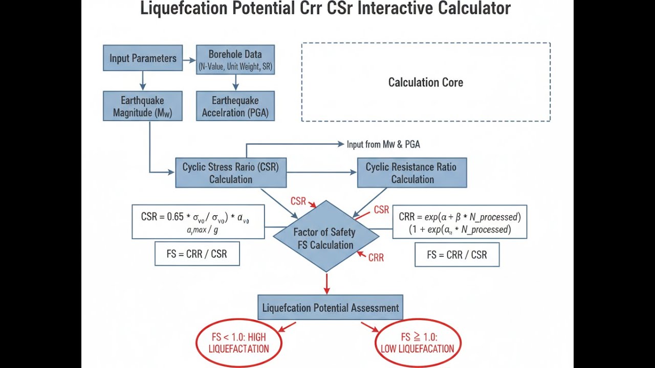
Diagram

Liquefaction Potential Calculator

Equations & Variables

Theory & Engineering Applications

Fundamental Mechanism of Liquefaction

Earthquake-induced liquefaction represents one of the most destructive soil failure mechanisms in geotechnical engineering. When saturated cohesionless soils experience cyclic loading from seismic shaking, the tendency for the soil skeleton to densify generates excess pore water pressure. If this pressure builds faster than it can dissipate through drainage, effective stress approaches zero, and the soil temporarily behaves as a viscous liquid rather than a solid. The simplified procedure pioneered by Seed and Idriss in 1971, and subsequently refined through decades of field performance data, provides the industry-standard framework for assessing this hazard.

The factor of safety against liquefaction compares the soil's cyclic resistance (CRR) to the earthquake-induced cyclic stress (CSR). A critical insight often overlooked is that this factor of safety represents a probability-based threshold rather than an absolute boundary. Field observations from the 1964 Niigata earthquake, the 1989 Loma Prieta earthquake, and the 2010-2011 Canterbury earthquake sequence demonstrate that sites with FS = 1.0 show approximately 50% probability of surface manifestation of liquefaction. Conservative practice typically targets FS ≥ 1.3 for critical structures, though this threshold depends on consequences of failure and uncertainty in input parameters.

Cyclic Stress Ratio Calculation and Physical Significance

The cyclic stress ratio quantifies the earthquake-induced shear stress normalized by the initial effective overburden stress. The coefficient 0.65 in the CSR equation represents the ratio of average cyclic shear stress to peak cyclic shear stress, derived from equivalent uniform loading concepts. This simplification allows complex irregular seismic loading to be represented by an equivalent uniform sinusoidal series of stress cycles. The stress reduction factor (r_d) accounts for the flexibility of the soil column—surface acceleration does not directly translate to equivalent base shaking throughout the profile due to soil deformability and wave propagation effects.

A non-obvious limitation emerges for sites with high static shear stress, such as sloping ground or beneath embankments. The simplified procedure was developed for level-ground conditions with minimal initial static shear. When static shear stress exceeds approximately 0.35 times the initial effective stress, flow failure can occur at lower cyclic stress levels than predicted by the standard equations. The Bray-Sancio procedure provides corrections for sloping ground, but these corrections become increasingly uncertain as static shear approaches the steady-state strength of the soil.

Cyclic Resistance from Standard Penetration Test Data

The cyclic resistance ratio represents the soil's ability to resist liquefaction, empirically correlated with the Standard Penetration Test (SPT) N-value corrected to 60% hammer energy efficiency and 100 kPa effective overburden stress. The relationship between N_160cs and CRR_7.5 was developed through extensive back-analysis of liquefaction case histories, plotting sites that did and did not liquefy during historical earthquakes. The boundary curves separating liquefied from non-liquefied sites provide the basis for the CRR equation.

The clean sand correction accounts for the increased resistance provided by non-plastic fines. Fine-grained soils require greater densification to achieve the same N-value as clean sands, meaning the same N-value indicates higher relative density and greater liquefaction resistance. However, this correction applies only to non-plastic or low-plasticity fines. When fines content exceeds 35% or plasticity index exceeds 12, the simplified procedure becomes invalid, and clay-like behavior dominates over liquefaction susceptibility.

Magnitude Scaling and Duration Effects

The reference earthquake magnitude in the original simplified procedure was M_w = 7.5, corresponding to approximately 15 equivalent uniform stress cycles. Smaller earthquakes produce fewer stress cycles, allowing greater cyclic resistance before liquefaction triggering. The magnitude scaling factor adjusts the resistance ratio to account for this duration effect. The Idriss (1999) MSF relationship replaced earlier linear correlations and shows MSF = 1.0 at M_w = 7.5, increasing to 1.8 for M_w = 6.0 and decreasing to 0.7 for M_w = 8.5.

An important practical consideration involves the selection of design earthquake magnitude. Deterministic seismic hazard analysis identifies the controlling earthquake scenario, while probabilistic analysis weights contributions from multiple magnitude-distance pairs. For sites where multiple scenarios contribute significantly to the hazard, using a single representative magnitude can unconservatively neglect the possibility that a larger, more distant earthquake could trigger liquefaction at depths where a smaller, closer event would not.

Fully Worked Example: Commercial Building Site Assessment

Consider a proposed three-story commercial building in Oakland, California, where SPT borings reveal saturated sandy soil at 6.0 m depth with the following properties: N₆₀ = 15 blows/0.3m, fines content FC = 12%, total unit weight γ = 19.2 kN/m³, and groundwater table at 3.0 m depth with γ_water = 9.81 kN/m³. The controlling earthquake scenario is M_w = 7.1 with peak ground acceleration a_max = 0.35g at the site.

Step 1: Calculate vertical stresses

Total vertical stress: σ_v = 19.2 kN/m³ × 6.0 m = 115.2 kPa

Pore water pressure: u = 9.81 kN/m³ × (6.0 - 3.0) m = 29.43 kPa

Effective vertical stress: σ'_v = 115.2 - 29.43 = 85.77 kPa

Step 2: Calculate stress reduction factor

At z = 6.0 m (less than 9.15 m): r_d = 1.0 - 0.00765(6.0) = 0.9541

Step 3: Calculate cyclic stress ratio

CSR = 0.65 × (0.35) × (115.2/85.77) × 0.9541 = 0.2772

Step 4: Calculate overburden correction factor

Since σ'_v = 85.77 kPa is less than 100 kPa:

K_σ = (85.77/100)^-0.5 = 1.0798

Step 5: Correct SPT N-value for fines content

For FC = 12% (between 5% and 35%):

α = exp(1.76 - 190/12²) = exp(1.76 - 1.319) = exp(0.441) = 1.554

β = 0.99 + (12^1.5/1000) = 0.99 + (41.57/1000) = 1.032

N_160cs = 1.554 + 1.032(15) = 1.554 + 15.48 = 17.03

Step 6: Calculate cyclic resistance ratio for M = 7.5

CRR_7.5 = (1/(34-17.03)) + (17.03/135) + (50/(10×17.03+45)²) - (1/200)

CRR_7.5 = (1/16.97) + 0.1261 + (50/215.3²) - 0.005

CRR_7.5 = 0.0589 + 0.1261 + 0.001078 - 0.005 = 0.1811

Step 7: Calculate magnitude scaling factor

MSF = 10^2.24 / 7.1^2.56 = 173.78 / 154.32 = 1.126

Step 8: Calculate final CRR and factor of safety

CRR = 0.1811 × 1.126 × 1.0798 = 0.2203

FS = CRR/CSR = 0.2203/0.2772 = 0.795

Engineering Assessment: With FS = 0.795, liquefaction is expected at this depth under the design earthquake. This site would require ground improvement (densification, drainage, or soil mixing) or a deep foundation system bypassing the liquefiable layer. The factor of safety is sufficiently below 1.0 that parameter uncertainty does not change the conclusion. At nearby depths with higher N-values or lower CSR, the assessment might yield FS closer to unity, where uncertainty analysis becomes critical.

Applications Across Engineering Disciplines

Liquefaction assessment extends beyond building foundation design into multiple critical applications. Transportation engineers evaluate bridge abutments and approach embankments where liquefaction-induced settlement creates dangerous transitions. The 1995 Kobe earthquake demonstrated catastrophic consequences when liquefaction beneath highway structures caused spans to collapse. Port facilities face particularly severe hazards because waterfront fill materials are often hydraulically placed loose sands, and lateral spreading toward open water faces can displace wharf structures by several meters.

Underground lifeline systems—water mains, sewer lines, natural gas pipelines—experience floatation and joint separation when surrounding soil liquefies. The buoyant force on a buried pipe can exceed gravitational resistance, causing pipelines to rise and rupture. Post-earthquake reconnaissance following the 2011 Christchurch earthquake documented extensive lifeline damage concentrated in areas of mapped liquefaction, with repair costs exceeding building damage in some neighborhoods. Modern practice includes liquefaction hazard mapping at city and regional scales, informing land-use planning, building code provisions, and infrastructure resilience strategies.

For additional engineering calculations and design tools, explore the comprehensive calculator library covering structural, mechanical, and geotechnical applications.

Practical Applications

Frequently Asked Questions