Aging equipment follows a predictable pattern: capital recovery costs drop as the initial investment spreads over more years, while operating and maintenance costs climb — and at some point, those two curves cross. That crossing point is your economic life, and getting it wrong costs real money. Use this Equipment Replacement Economic Life Calculator to calculate the optimal replacement year and equivalent annual cost (EAC) using initial cost, salvage decline rate, operating cost growth, and discount rate. It matters across fleet management, heavy manufacturing, mining, and any capital-intensive operation where equipment replacement timing drives budget performance. This page includes the EAC and CRF formulas, a worked industrial example, defender vs. challenger analysis theory, and a full FAQ.
What is equipment economic life?
Equipment economic life is the number of years you should own a piece of equipment before replacing it — specifically, the point where your total annual ownership cost (capital plus operating) is at its lowest. Hold it longer and rising maintenance costs push your annual cost back up.
Simple Explanation
Think of it like a car: brand new, it's expensive to buy but cheap to run. Ten years on, it's nearly paid off but nickel-and-diming you with repairs every few months. Economic life is the sweet spot — the age where those two pressures balance out and your total yearly cost is as low as it gets. The calculator finds that sweet spot for your equipment automatically.
📐 Browse all 1000+ Interactive Calculators
Visual Diagram

How to Use This Calculator
- Select your calculation mode from the dropdown — Economic Life & EAC, Challenger vs. Defender, Operating Cost Projection, or Salvage Value Declining Balance.
- Enter your equipment's initial cost, discount rate, initial salvage value, salvage decline rate, first-year operating cost, operating cost growth rate, and maximum analysis period.
- Adjust any values to match your specific equipment profile — use real purchase prices, actual maintenance records, and your organization's cost of capital.
- Click Calculate to see your result.
Equipment Replacement Economic Life Calculator
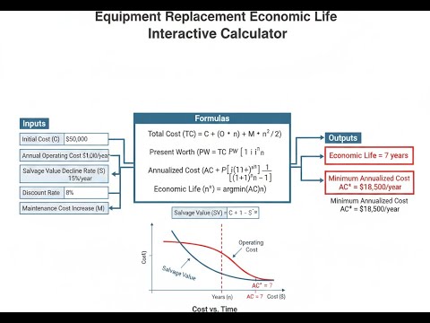
Equipment Replacement Economic Life Interactive Calculator
Visualize how capital recovery costs drop while operating costs rise over equipment lifetime. Watch the crossing point reveal optimal replacement timing for minimum equivalent annual cost.
ECONOMIC LIFE
7 years
MIN EAC
$16,420
CAPITAL COST
$8,940
OPERATING COST
$7,480
FIRGELLI Automations — Interactive Engineering Calculators
Economic Life Equations
Use the formula below to calculate equivalent annual cost (EAC).
Equivalent Annual Cost (EAC)
EAC = NPV × CRF
Where:
- NPV = Net Present Value of total ownership costs over equipment life ($)
- CRF = Capital Recovery Factor (dimensionless)
- EAC = Equivalent Annual Cost, expressing total costs as uniform annual amount ($/year)
Capital Recovery Factor
CRF = [r(1 + r)n] / [(1 + r)n - 1]
Where:
- r = Discount rate per period (decimal)
- n = Number of periods (years)
- CRF = Converts present value to equivalent annuity (1/year)
Net Present Value of Ownership
NPV = -P + Sn/(1+r)n - Σ[Ot/(1+r)t]
Where:
- P = Initial purchase price or current market value ($)
- Sn = Salvage value at end of year n ($)
- Ot = Operating and maintenance cost in year t ($/year)
- t = Year index from 1 to n
- Σ = Summation over all years of ownership
Salvage Value Declining Balance
Sn = S0(1 - d)n
Where:
- S0 = Initial salvage value (often purchase price minus installation) ($)
- d = Depreciation rate per period (decimal)
- n = Age of equipment (years)
- Sn = Salvage or market value after n years ($)
Operating Cost Growth Model
Ot = O1(1 + g)t-1
Where:
- O1 = Operating cost in first year ($/year)
- g = Annual growth rate in operating costs (decimal)
- t = Year number (t = 1, 2, 3, ...)
- Ot = Operating cost in year t ($/year)
Simple Example
Equipment purchase price: $50,000. First-year operating cost: $5,000, growing 10% per year. Salvage value starts at $40,000, declining 20% per year. Discount rate: 8%.
- Year 3 salvage: $40,000 × (0.80)³ = $20,480
- PV of 3 years' operating costs ≈ $12,800
- NPV = −$50,000 + $16,256 − $12,800 = −$46,544
- EAC (Year 3) ≈ $18,100/year
- Running this across years 1–10 finds the year where EAC is lowest — that's your economic life.
Theory & Engineering Applications
Economic life analysis addresses a fundamental challenge in capital asset management: determining when to replace equipment to minimize total ownership costs. Unlike physical life—how long equipment can operate—or technological life—how long it remains competitive—economic life represents the optimal ownership period where the equivalent annual cost reaches its minimum value. This occurs at the intersection of two opposing cost trajectories: declining capital recovery costs (as the initial investment is amortized over more years) and rising operating costs (as aging equipment becomes less efficient and requires more maintenance).
The Equivalent Annual Cost Framework
The EAC methodology transforms all costs associated with equipment ownership—initial purchase, operating expenses, maintenance, and final salvage value—into a uniform annual equivalent. This approach enables valid comparisons between alternatives with different lifespans, cost structures, and timing patterns. The fundamental principle relies on the time value of money: a dollar today is worth more than a dollar in the future due to opportunity cost represented by the discount rate. For capital-intensive industries, the discount rate typically reflects the weighted average cost of capital (WACC), which combines debt and equity financing costs weighted by their proportions in the firm's capital structure.
A critical non-obvious aspect of economic life calculations is the sensitivity to operating cost growth rates. Small variations in the annual increase of maintenance and operating expenses can shift the optimal replacement point by several years. For example, equipment experiencing 12% annual cost growth versus 18% growth might show a two-year difference in economic life, dramatically affecting total cost of ownership. This sensitivity stems from the geometric compounding of cost increases—a phenomenon that accelerates non-linearly as equipment ages beyond its design life.
Challenger-Defender Replacement Analysis
Real-world replacement decisions involve comparing a "defender" (current equipment) against a "challenger" (potential replacement). The defender's first cost is its current market value, not its original purchase price or book value—a crucial distinction that many practitioners miss. Sunk costs are irrelevant to forward-looking economic decisions. The proper comparison equates the EAC of keeping the defender for its remaining optimal life against the EAC of acquiring and operating the challenger for its economic life.
This framework reveals an important limitation: it assumes repeated cycles of identical replacements into perpetuity. In reality, technology improvements may make future challengers more attractive, introducing option value to delaying replacement. The analysis also assumes accurate forecasting of future operating costs and salvage values—predictions that become increasingly uncertain beyond 3-5 years for most industrial equipment. Sensitivity analysis across ranges of key parameters becomes essential for robust decision-making.
Present Value Calculations and Discount Rate Selection
The discount rate profoundly influences economic life calculations. Higher discount rates place less weight on distant future costs, generally shortening calculated economic life because near-term operating cost increases have greater impact than distant salvage value. For publicly traded companies, discount rates typically range from 7% to 15% depending on industry risk, leverage, and market conditions. Government entities and utilities often use lower social discount rates (3% to 7%), reflecting longer time horizons and different risk profiles. Using a nominal discount rate requires expressing all cash flows in nominal dollars (including inflation), while real discount rates pair with real cash flows.
The capital recovery factor converts the net present value of ownership into an equivalent annuity. Mathematically, CRF equals the payment on a loan of $1 at interest rate r for n periods. This relationship makes intuitive sense: owning equipment is economically equivalent to borrowing its net cost (purchase minus present value of salvage) at the discount rate. The CRF decreases as equipment life increases, reflecting the benefit of spreading capital costs over more years—but only up to the point where increasing operating costs offset this benefit.
Worked Example: Industrial Forklift Replacement Analysis
Consider a manufacturing facility evaluating replacement timing for a fleet of electric forklifts. A new forklift costs $47,500 with expected first-year operating costs of $8,200 including electricity, routine maintenance, and operator training. Operating costs increase 13.5% annually due to battery degradation, increased maintenance needs, and reduced efficiency. The discount rate is 9.2% reflecting the company's WACC. Initial salvage value equals purchase price minus $2,500 for delivery and setup, giving $45,000. Salvage value declines 22% per year based on dealer trade-in quotations for aging units.
Step 1: Calculate salvage values for years 1-10
- Year 1: S₁ = $45,000 × (1 - 0.22)¹ = $45,000 × 0.78 = $35,100
- Year 2: S₂ = $45,000 × (0.78)² = $45,000 × 0.6084 = $27,378
- Year 3: S₃ = $45,000 × (0.78)³ = $45,000 × 0.4746 = $21,357
- Year 4: S₄ = $45,000 × (0.78)⁴ = $45,000 × 0.3702 = $16,659
- Year 5: S₅ = $45,000 × (0.78)⁵ = $45,000 × 0.2887 = $12,991.50
- Year 6: S₆ = $45,000 × (0.78)⁶ = $45,000 × 0.2252 = $10,134
Step 2: Calculate present value of operating costs for n = 5 years
- Year 1: O₁ = $8,200 / (1.092)¹ = $8,200 / 1.092 = $7,509.89
- Year 2: O₂ = $8,200 × 1.135 / (1.092)² = $9,307 / 1.192464 = $7,804.73
- Year 3: O₃ = $8,200 × (1.135)² / (1.092)³ = $10,563.45 / 1.302171 = $8,113.92
- Year 4: O₄ = $8,200 × (1.135)³ / (1.092)⁴ = $11,989.52 / 1.421970 = $8,431.89
- Year 5: O₅ = $8,200 × (1.135)⁴ / (1.092)⁵ = $13,608.10 / 1.552791 = $8,763.72
- Total PV Operating (5 years) = $40,624.15
Step 3: Calculate NPV and EAC for n = 5 years
- PV of salvage: $12,991.50 / (1.092)⁵ = $12,991.50 / 1.552791 = $8,366.22
- NPV = -$47,500 + $8,366.22 - $40,624.15 = -$79,757.93
- CRF = [0.092 × (1.092)⁵] / [(1.092)⁵ - 1] = 0.142848 / 0.552791 = 0.2585
- EAC = -(-$79,757.93) × 0.2585 = $20,616.53 per year
Step 4: Repeat for years 1-10 to find minimum EAC
Following identical procedures for each year from 1 to 10, the calculated EAC values are:
- Year 1: $21,273.64 | Year 2: $19,847.21 | Year 3: $19,256.33 | Year 4: $19,184.29 | Year 5: $19,443.82 (minimum near here)
- Year 6: $19,897.44 | Year 7: $20,473.29 | Year 8: $21,132.85 | Year 9: $21,851.76 | Year 10: $22,614.92
Result: The economic life is approximately 4 years where EAC reaches its minimum of $19,184.29. At this point, the forklift should be replaced. Keeping it beyond 4 years results in higher equivalent annual costs due to accelerating operating expenses and diminishing salvage value. This analysis assumes the company can continuously replace with identical equipment—if next-generation forklifts offer significantly better economics, replacement might be justified even earlier.
Industry-Specific Applications
In mining operations, haul truck economic life typically ranges from 5-8 years depending on utilization intensity and ore characteristics. Abrasive materials accelerate wear, shortening economic life despite manufacturers' 15-20 year design life claims. Transportation fleets managing thousands of vehicles use economic life models with real-time telematics data to predict optimal replacement schedules, reducing total fleet costs by 8-15% compared to arbitrary age-based policies.
Manufacturing facilities apply economic life analysis to production equipment where downtime costs create asymmetric risk—the cost of unexpected failure far exceeds planned replacement expense. This introduces a reliability constraint: replacement may be justified before reaching minimum EAC if failure probability exceeds acceptable thresholds. Semiconductor fabrication plants exemplify this extreme case, where $500,000 process tools might be replaced after just 3-4 years despite 10-year economic life calculations, driven by rapidly advancing lithography technology and product yield improvements.
For more engineering economics tools and financial analysis calculators, explore the comprehensive engineering calculator library.
Practical Applications
Scenario: Municipal Fleet Manager Optimizing Bus Replacement
Marcus, the fleet manager for a mid-sized city transit system, oversees 85 diesel buses with ages ranging from 2 to 14 years. The city council is pressuring him to extend vehicle life to 15 years to reduce capital expenditures, but he suspects this is false economy. Using the economic life calculator, Marcus inputs data for their newest bus model: $425,000 purchase price, $62,000 first-year operating costs (fuel, maintenance, insurance), 11% annual operating cost increase based on historical maintenance records, 18% salvage value decline, and 7.5% municipal discount rate. The calculator reveals an economic life of 9 years with minimum EAC of $138,450, while forcing buses to 15 years increases EAC to $171,230—costing the city an extra $32,780 per bus annually. Armed with this quantitative analysis showing $2.78 million in annual excess costs across the fleet, Marcus successfully advocates for the optimal 9-year replacement cycle in the next budget presentation.
Scenario: Construction Company Evaluating Excavator Upgrade
Jennifer runs a commercial excavation contractor with five hydraulic excavators, the oldest being a 6-year-old 320-ton unit purchased for $287,000. A dealer offers $94,000 trade-in value and proposes a new fuel-efficient model at $338,000 with 22% better fuel economy and advanced telematics reducing maintenance costs. She uses the challenger-defender calculator mode, inputting defender values (current market $94,000, annual operating costs $47,500, 4-year remaining life, $28,000 final salvage) versus challenger specifications (purchase $338,000, operating costs $36,200 thanks to efficiency gains, 8-year economic life, $89,000 salvage). At their 10.2% cost of capital, the calculator shows defender EAC of $75,920 versus challenger EAC of $84,140—suggesting she should keep the current excavator for now. However, the analysis reveals that if fuel prices increase just 15% or the defender's operating costs rise to $52,000 (well within normal variance), the challenger becomes economically superior. This insight prompts Jennifer to monitor actual costs quarterly and pre-negotiate pricing with the dealer for replacement within the next 12-18 months when economics will likely favor the upgrade.
Scenario: Hospital Biomedical Engineer Planning MRI Replacement Budget
Dr. Chen, the biomedical engineering director at a regional hospital, must forecast replacement timing for their $2.1 million 3-Tesla MRI scanner currently in its fourth year of operation. Hospital CFO demands a 10-year capital equipment plan with defendable numbers for the board. Dr. Chen knows from vendor service records that MRI operating costs—including helium refills, preventive maintenance contracts, repairs, and cooling system electricity—start at $185,000 annually but increase 8.5% per year as components age and service contract costs escalate. Using market data from similar hospitals, she estimates 12% annual salvage value decline from initial resale value of $1.8 million, with the hospital's 6.8% cost of capital. The calculator projects an 11-year economic life with minimum EAC of $487,320. However, Dr. Chen also knows that imaging technology improvements follow a rapid curve—next-generation scanners will offer superior diagnostic capabilities in 7-8 years. She presents the board with two scenarios: pure economic replacement at year 11 versus technology-driven replacement at year 8, showing the premium of $38,000 annually for earlier adoption of superior imaging technology. This structured analysis enables an informed strategic decision balancing cost minimization with maintaining competitive clinical capabilities.
Frequently Asked Questions
Free Engineering Calculators
Explore our complete library of free engineering and physics calculators.
Browse All Calculators →🔗 Explore More Free Engineering Calculators
About the Author
Robbie Dickson — Chief Engineer & Founder, FIRGELLI Automations
Robbie Dickson brings over two decades of engineering expertise to FIRGELLI Automations. With a distinguished career at Rolls-Royce, BMW, and Ford, he has deep expertise in mechanical systems, actuator technology, and precision engineering.
Need to implement these calculations?
Explore the precision-engineered motion control solutions used by top engineers.


