Life Cycle Cost Ownership Interactive Calculator

The Life Cycle Cost (LCC) calculator enables engineers, procurement specialists, and financial analysts to evaluate the total cost of ownership for equipment, systems, or projects from initial acquisition through disposal. Unlike simple purchase price comparisons, LCC analysis accounts for acquisition costs, operating expenses, maintenance, downtime, energy consumption, and end-of-life disposal to reveal the true economic impact of capital investment decisions across industries from manufacturing to infrastructure development.

📐 Browse all free engineering calculators

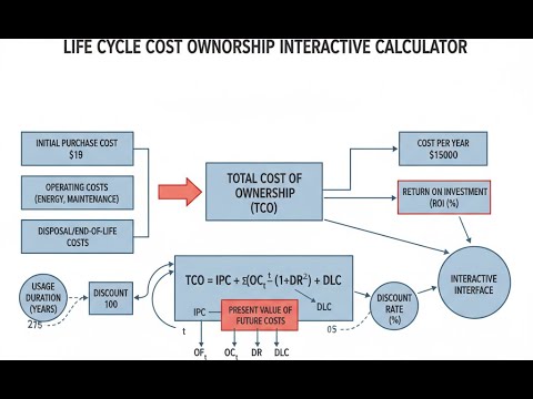
Visual Diagram: Life Cycle Cost Components

Life Cycle Cost Ownership Calculator

Formulas & Life Cycle Cost Equations

Theory & Engineering Applications of Life Cycle Costing

Life cycle cost analysis represents a comprehensive economic evaluation methodology that extends far beyond simple acquisition price comparison. Engineering decisions made during procurement affect operational expenses, maintenance requirements, energy consumption, and disposal costs for decades. A manufacturing facility purchasing a $100,000 compressor system with 85% energy efficiency versus a $140,000 unit at 93% efficiency demonstrates this principle—over a 20-year service life operating 6,000 hours annually at $0.12/kWh for a 75 kW motor, the higher-efficiency unit saves approximately $108,000 in energy costs alone, making it the economical choice despite the 40% higher purchase price.

Time Value of Money and Discount Rate Selection

The discount rate fundamentally transforms LCC analysis from simple arithmetic to sophisticated financial modeling. This rate reflects opportunity cost, inflation, and risk, converting future expenditures to present value equivalents. Federal agencies typically use 3-7% discount rates for public infrastructure, while private corporations may apply 10-15% rates reflecting shareholder return expectations and capital costs. The choice profoundly impacts decision-making: at 3% discount, a $50,000 expense 15 years hence has a present value of $32,076, but at 10% it drops to $11,970. This explains why high discount rates favor lower initial costs with higher operating expenses—future costs become heavily discounted. Defense procurement often uses lower rates (2-4%) because assets serve national security over 30-50 year horizons, while technology equipment uses higher rates (12-18%) reflecting rapid obsolescence and 3-5 year replacement cycles.

Hidden Cost Categories in Industrial Systems

Downtime costs frequently exceed all other operating expenses in production environments yet remain poorly quantified in many LCC analyses. A pharmaceutical filling line generating $18,000 per hour in finished product value experiences true downtime costs of $18,000/hour plus labor, material waste, and schedule disruption—often totaling $25,000-$30,000 per hour. Reliability-centered maintenance principles suggest that equipment with 99.2% availability versus 97.5% availability operating 8,760 hours annually creates 149 hours versus 219 hours of downtime—a 70-hour differential. At $25,000/hour, this represents $1.75 million in annual value difference, justifying substantial initial cost premiums for higher-reliability equipment. This calculation method applies across automotive assembly, semiconductor fabrication, and food processing where line stoppages cascade through integrated production systems.

Energy Cost Escalation and Long-Term Projections

Historical energy price volatility introduces significant uncertainty into LCC calculations for energy-intensive equipment. U.S. industrial electricity prices increased from $0.0483/kWh in 2000 to $0.0712/kWh in 2023—a 47% rise over 23 years, or approximately 1.7% annual escalation above inflation. Conservative LCC analyses incorporate energy escalation rates of 2-3% annually above the general discount rate. For a data center consuming 2.5 MW continuously, the difference between flat energy costs and 2.5% annual escalation over 15 years equals $8.7 million in additional expenses (assuming $0.08/kWh baseline). Variable frequency drives, high-efficiency motors, heat recovery systems, and LED lighting retrofits all demonstrate enhanced economic justification when energy escalation factors enter the analysis. Process industries performing LCC analysis should separate energy costs from other operating expenses and apply sector-specific escalation rates based on fuel type—natural gas, electricity, or diesel—each following distinct price trajectories.

Worked Example: HVAC System Selection for Commercial Building

A 150,000 square foot office building in Chicago requires HVAC replacement. Two systems warrant evaluation:

Option A: Standard Efficiency System
Initial equipment cost: $385,000
Installation cost: $95,000
Annual energy consumption: 1,850,000 kWh at $0.095/kWh = $175,750/year
Annual maintenance: $18,500
Service life: 18 years
Salvage value: $12,000

Option B: High Efficiency System with Heat Recovery
Initial equipment cost: $565,000
Installation cost: $115,000
Annual energy consumption: 1,295,000 kWh at $0.095/kWh = $123,025/year
Annual maintenance: $24,750
Service life: 22 years
Salvage value: $28,000

Using 5% discount rate and 2% annual energy cost escalation, we calculate NPV for each option over an 18-year common analysis period (Option A's full life):

Option A Calculations:
Initial costs: $385,000 + $95,000 = $480,000
Year 1 operating cost: $175,750 + $18,500 = $194,250
Year 2 operating cost: ($175,750 × 1.02) + $18,500 = $197,758
Continuing this pattern through year 18, then discounting each year's cost to present value using the formula: PV = Cost / (1.05)^year

Summing all present values:
PV of operating costs (years 1-18): $2,847,365
PV of salvage value: $12,000 / (1.05)¹⁸ = $4,992
Total LCC (Option A): $480,000 + $2,847,365 - $4,992 = $3,322,373

Option B Calculations:
Initial costs: $565,000 + $115,000 = $680,000
Year 1 operating cost: $123,025 + $24,750 = $147,775
Year 2 operating cost: ($123,025 × 1.02) + $24,750 = $150,236
Following the same discounting methodology through year 18:
PV of operating costs (years 1-18): $2,174,483
Total LCC (Option B, 18-year analysis): $680,000 + $2,174,483 = $2,854,483

Economic Comparison:
Net savings with Option B: $3,322,373 - $2,854,483 = $467,890
Savings as percentage: 14.1% over analysis period
Simple payback period: ($680,000 - $480,000) / ($194,250 - $147,775) = 4.3 years
Discounted payback: Approximately 5.1 years (accounting for time value)

This analysis reveals that despite a $200,000 higher initial investment (41.7% premium), Option B delivers nearly $468,000 in present value savings over 18 years. The energy savings of $52,725/year in year one, escalating at 2% annually, compound to create overwhelming economic advantage. Additionally, Option B's 22-year service life versus 18 years provides four additional years of service value not captured in this conservative 18-year analysis window.

Maintenance Cost Modeling and Equipment Aging

Constant annual maintenance costs represent an oversimplification in most LCC models. Real-world maintenance expenses follow escalating patterns as equipment ages—hydraulic systems develop seal leaks, bearings wear, control systems require reprogramming, and component obsolescence forces expensive retrofits. A realistic maintenance cost model uses a bathtub curve with three phases: early life (infant mortality), stable operation, and wear-out period. Industrial pumps typically show stable maintenance years 3-10, then 8-12% annual cost increases through year 20. A pump with $4,000 annual maintenance years 3-10 might require $4,320 in year 11, $4,666 in year 12, escalating to $8,200 by year 20. Incorporating this realistic cost progression into LCC analysis increases total costs by 15-22% compared to flat-rate models, favoring equipment replacement at optimal economic life rather than running assets to failure.

Sensitivity Analysis and Monte Carlo Simulation

LCC calculations contain multiple uncertain variables—discount rates, energy prices, maintenance costs, equipment lifespans, and utilization rates—each affecting outcomes. Deterministic single-point estimates mask this uncertainty. Sophisticated LCC analysis employs sensitivity analysis, varying each parameter individually to identify which variables most impact decision-making. A tornado diagram ranks parameters by influence magnitude. For major capital decisions, Monte Carlo simulation runs 10,000+ iterations with probability distributions for each variable, generating a distribution of possible LCC outcomes rather than single values. This reveals that "Option A: $2.85M" might actually represent a 90% confidence interval of $2.31M to $3.67M, while "Option B: $3.22M" spans $2.89M to $3.58M—potentially reversing the decision when uncertainty is properly quantified. Risk-averse organizations might select the option with lower worst-case outcome even if mean costs are higher.

For those performing comparative economic analysis across multiple options, the engineering calculator library offers additional tools for payback period calculation, internal rate of return, and benefit-cost ratio analysis that complement LCC methodology.

Practical Applications

Frequently Asked Questions