Safety Stock Statistical Interactive Calculator

Stockouts usually come down to two culprits: unpredictable demand and suppliers who take longer than expected to deliver. If you try to eyeball your buffer inventory, you’ll either waste money or risk running dry. The Safety Stock Statistical Calculator here works out buffer inventory using the actual numbers that matter—the service level you want, how wild your demand is, and how much lead time can swing. This isn’t just theoretical. It’s useful anywhere a stockout will cost you time or customers, whether you’re on a factory floor, filling shelves, or running a distribution center. Below you’ll find the working equations, an example run-through, where the statistics really matter, and a detailed FAQ.

What is Safety Stock?

Safety stock is the extra inventory you hold to cover for unexpected surges in demand or for late supplier deliveries—anything above what you’d expect to need while waiting for an order to arrive. It’s meant to stop production or sales from grinding to a halt when things don’t go according to plan.

Simple Explanation

Safety stock is your backup—like keeping a spare tire in the trunk. Most days, you won’t need it, but it saves you when you hit a rough patch: demand pops up higher than average, or your order gets stuck somewhere. The rougher or more uncertain things get (either demand or delivery), the more backup you’ll need, plain and simple.

📐 Browse all 1000+ Interactive Calculators

How to Use This Calculator

1. Pick your calculation: Basic Safety Stock, Variable Lead Time, Reorder Point, or a reverse calculation.
2. Put in your numbers—average demand, demand’s standard deviation, average lead time, and service level (or the number you’re solving for).
3. If you’re using Variable Lead Time, add the standard deviation for lead time too.
4. Hit Calculate to see the answer.

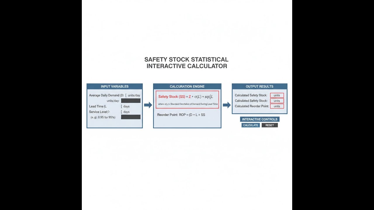
Diagram

Safety Stock Statistical Calculator

Equations & Formulas

Below is the standard approach for safety stock when lead time doesn't swing.

When both your demand and your lead time bounce around, use this one instead.

If you want the reorder point, base it on average demand, lead time, and the calculated safety stock:

Standard deviation during the lead time isn't always obvious—here’s how you figure it out:

Simple Example

Average daily demand: 100 units
Standard deviation of demand: 20 units/day
Average lead time: 7 days
Target service level: 95% → Z-score = 1.645
σ during lead time = 20 × √7 = 52.92 units
Safety Stock = 1.645 × 52.92 = 87.06 units

Theory & Engineering Applications

Safety stock is your working buffer against uncertainty—an extra layer above what you’d expect to go through during lead time. It’s not based on gut feeling; the idea is to handle real-life swings in usage and delays. Older, deterministic approaches assume you know exactly what you’ll need and when. That rarely happens. Using these statistical methods, you’re actually putting a number on your risk rather than guessing, which makes sense when stakes are high or you’ve been burned by guesswork in the past.

Fundamental Statistical Principles

Safety stock formulas generally assume that total demand over your lead time behaves like a normal distribution. That assumption can be off for niche or highly variable items, but it holds up decently for high-volume parts where randomness averages out. Z-score isn’t just math jargon—it tells you how far you’re padding above average demand for the service level you want. For example, a 95% service level means carrying enough inventory to cover average demand plus another 1.645 standard deviations’ worth of surprises. That leaves roughly a 5% chance you’ll run out.

Be aware: ‘standard deviation of demand’ tells you how much your day-to-day usage jumps around, not how far off your forecasts are. Many make the mistake of building forecast error into their safety stock calculation, which ends up double-counting uncertainty. You’ll get more inventory than you need and pay for it. If you find a chronic gap between forecast and reality, use that to fix your forecasting method, not as a reason to keep stockpiling.

Variable Lead Time Complexity

When lead time itself is unpredictable, you need a formula that can handle both moving targets: demand and delivery. The total variance during lead time is the sum of two things: how much demand varies, multiplied by average lead time, and how much lead time varies, scaled up by average demand squared. This means that if your demand number is high, even moderate swings in lead time create huge uncertainty and can swamp the effect of variable demand. For example, a big manufacturer using 10,000 units a day and seeing swings of just a day or two in lead time is in a much riskier position than a small supplier with slow-moving stock, even if delivery uncertainty is the same.

These formulas assume demand and lead time don’t influence each other—often not the case. When things get busy, suppliers can slip behind, so spikes in demand and delays actually happen together. If you see that in your business, you’ll need to adjust: bump up your safety stock by a quarter or so over the calculated number (plus or minus), or run some historical simulations if you need to be more exact. There’s no perfect one-size-fits-all math for correlation without more advanced modelling.

Service Level Interpretation and Cost Trade-offs

‘Service level’ means different things depending on who’s asking. Most formulas here target the chance of a stockout per cycle, but your boss might care more about the percentage of actual orders you can fill from stock. These aren't always the same—especially when you’re dealing with items that don’t move much but have unpredictable spikes. The disconnect can lead to the wrong stocking policy if you’re not careful.

The sweet spot for service level is where the cost of carrying more inventory equals the cost of running out. In the real world, that’s a slog to calculate, since runout costs depend on lost sales, angry customers, extra shipping, and so on—and these costs are hard to pin down. Most companies pick some global targets (e.g. 95% for important items) and move on. Better practice is to break stock into categories (fast movers, slow movers, high value, etc.) and tune service levels to what actually makes sense for each.

Practical Calculation Example: Medical Device Distribution

Here’s a relatable scenario. Say you oversee inventory for surgical staplers. You see average daily demand of 87 units (standard deviation: 23). Your supplier usually takes 42 days, but it can swing by 6 days. Targeting a 98% service level, find the Z-score: it’s 2.054. Calculate combined variance: (42 × 23²) + (87² × 6²). That’s (42 × 529) + (7569 × 36) = 22,218 + 272,484 = 294,702. The standard deviation during lead time is the square root: 542.87 units. Multiply by Z: safety stock is about 1,115 units. Your reorder point becomes average demand during lead time (87 × 42 = 3,654 units) plus safety stock, so 4,769 units. Notice how the lead time variation (supplier’s side) dominates most of the total uncertainty—if you can reduce that, your safety stock requirements drop fast. For example, halving the lead time swing almost cuts required safety stock by 35%.

Advanced Considerations in Modern Supply Chains

Classic formulas assume average demand and its swings aren’t shifting. In practice, demand can trend up, crash, or whipsaw seasonally—think new product launches or holiday surges. If you use an old average and variance for something that’s growing, you’ll get stockouts. If the product is dying off, you’ll be loaded up with dead inventory. To tackle this, keep your safety stock stats current: for fast-changing products, use shorter history windows, and update frequently. For steady products, longer time frames will do.

When you hold stock in more than one location—like a warehouse and a bunch of stores—blindly adding safety stock everywhere quickly stacks up. Multi-echelon inventory models handle this by pooling risk: holding more at a central spot and less elsewhere, cutting down on total buffer but still covering uncertainty across the network. This only works if your locations actually share risk (they pull from the same central supply and demand isn’t perfectly synchronized at the edges). For a more hands-on approach to tuning safety stock for your own setup, see our engineering calculator library.

Practical Applications

Frequently Asked Questions

Video Walkthrough - How to Use This Calculator