Comparing capital investments with different lifespans, irregular cash flows, and varying upfront costs is one of the trickier problems in engineering economics — standard cost comparisons break down fast when project lives don't match. Use this Annual Worth Calculator to calculate the equivalent uniform annual value of any investment using initial cost, annual benefits and costs, salvage value, interest rate, and project life. It matters in infrastructure planning, manufacturing equipment selection, energy systems, and fleet management, where annual budget alignment is as important as raw economics. This page includes the core AW formula, a worked solar installation example, theory on handling unequal lives, and a full FAQ covering inflation, tax effects, and discount rate selection.
What is Annual Worth?
Annual Worth (AW) is a method of expressing all the costs and benefits of an investment as a single equivalent dollar amount per year. If a project has a positive AW, it returns more value each year than it costs — it's worth doing.
Simple Explanation
Think of AW like converting a mortgage into a monthly payment — instead of one big number, you spread everything out evenly across the life of the investment. You take the upfront cost, the ongoing expenses, any future salvage value, and all the benefits, then ask: "What's the net value per year, in today's money?" If that number is positive, the project pays off. If it's negative, it doesn't.
📐 Browse all 1000+ Interactive Calculators
Annual Worth Cash Flow Diagram

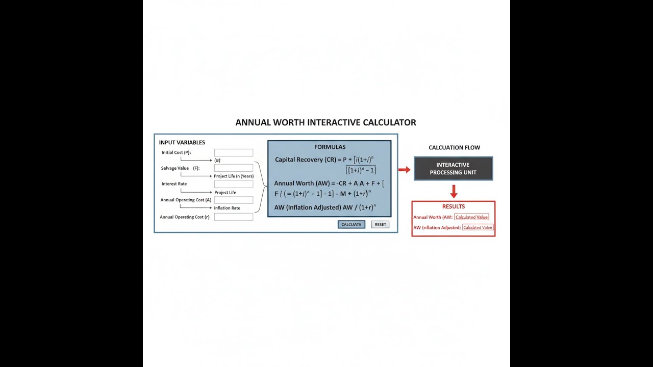
Annual Worth Interactive Calculator
How to Use This Calculator
- Select a Calculation Mode from the dropdown — choose from single project AW, compare two alternatives, capital recovery, perpetual AW, gradient series, or required salvage value.
- Enter your project inputs: initial cost, annual benefit, annual cost, salvage value, interest rate, and project life (fields shown will match your selected mode).
- Use the "Try Example" button to load pre-filled values and see a live result before entering your own data.
- Click Calculate to see your result.
Annual Worth Interactive Visualizer
Watch how initial cost, annual cash flows, and salvage value combine to create equivalent uniform annual worth. Adjust parameters to see real-time impact on project acceptability and economic efficiency.
ANNUAL WORTH
$1,065
CAPITAL RECOVERY
$9,372
NET ANNUAL
$10,000
FIRGELLI Automations — Interactive Engineering Calculators
Key Annual Worth Equations
Use the formula below to calculate Annual Worth.
Basic Annual Worth Formula
AW = Abenefits - Acosts - P(A/P, i, n) + S(A/F, i, n)
Where:
- AW = Annual Worth ($/year)
- Abenefits = Annual benefits or revenues ($/year)
- Acosts = Annual operating and maintenance costs ($/year)
- P = Initial investment or present cost ($)
- S = Salvage value at end of project life ($)
- i = Interest rate per period (decimal)
- n = Number of periods (years)
Capital Recovery Factor (CRF)
(A/P, i, n) = [i(1 + i)n] / [(1 + i)n - 1]
Converts a present amount to an equivalent uniform annual series. This factor answers: "What annual payment is needed to recover an investment P over n periods at interest rate i?"
Sinking Fund Factor (SFF)
(A/F, i, n) = i / [(1 + i)n - 1]
Converts a future amount to an equivalent uniform annual series. Used to determine the annual equivalent of salvage value or future receipts.
Arithmetic Gradient Factor (AGF)
(A/G, i, n) = (1/i) - n / [(1 + i)n - 1]
Converts an arithmetic gradient series (where cash flows increase by constant amount G each period) to an equivalent uniform annual series. Used when costs or benefits change linearly over time.
Perpetual Annual Worth
AWperpetual = A - Pi
For projects with infinite life (n → ∞), the capital recovery simplifies to the annual interest on the initial investment. Applicable to endowments, long-lived infrastructure, and perpetual investments.
Simple Example
You invest $50,000 in a piece of equipment, earn $12,000/year in benefits, spend $2,000/year in operating costs, expect a $5,000 salvage value after 8 years, and your interest rate is 10%.
- CRF = [0.10 × (1.10)⁸] / [(1.10)⁸ − 1] = 0.18744
- SFF = 0.10 / [(1.10)⁸ − 1] = 0.08744
- AW = $12,000 − $2,000 − ($50,000 × 0.18744) + ($5,000 × 0.08744)
- AW = $10,000 − $9,372 + $437 = +$1,065/year — project is acceptable.
Theory & Engineering Applications of Annual Worth Analysis
Annual Worth (AW) analysis represents one of the fundamental pillars of engineering economics, providing a robust methodology for evaluating capital investments by converting all cash flows—both initial investments and future receipts—into an equivalent uniform annual series. This transformation enables direct comparison of alternatives with different lifespans, irregular cash flow patterns, and varying capital requirements. The AW method proves particularly valuable when comparing mutually exclusive alternatives, as it naturally handles the common engineering situation where options have different useful lives without requiring least common multiple assumptions.
Theoretical Foundation and Economic Interpretation
The annual worth of a project represents the equivalent uniform annual value that, if received or paid every year over the project life, would be economically equivalent to the actual cash flow pattern at a specified interest rate. Unlike Present Worth (PW) analysis which collapses all cash flows to time zero, or Future Worth (FW) which projects to the end of the study period, AW distributes the economic value uniformly across the project timeline. This distribution aligns naturally with organizational budgeting processes and operating expense frameworks, making AW particularly intuitive for decision-makers who think in terms of annual budgets, quarterly earnings, and fiscal year performance.
The Capital Recovery Factor (CRF) embedded in AW calculations embodies a critical economic concept: it simultaneously accounts for both capital recovery and the opportunity cost of funds. When you multiply an initial investment P by the factor (A/P, i, n), you determine the annual payment required to recover that investment while providing the required return i over n periods. The CRF increases with higher interest rates and decreases with longer project lives, reflecting the fundamental time value of money. For a $100,000 investment at 10% over 10 years, the CRF equals 0.16275, meaning $16,275 must be recovered annually. This exceeds the simple principal recovery ($10,000/year) by $6,275 annually to compensate for the opportunity cost of capital.
Handling Unequal Project Lives: The AW Advantage
One of the most powerful features of Annual Worth analysis emerges when comparing alternatives with different useful lives. Consider comparing a $50,000 machine with a 6-year life to an $80,000 machine with a 10-year life. Present Worth analysis requires assuming repeated replacement cycles over a least common multiple period (30 years in this case), creating computational complexity and introducing questionable assumptions about future replacement costs and technologies. Annual Worth elegantly sidesteps this issue: each alternative is evaluated over its own life, and the resulting AW values can be directly compared. This works because AW implicitly assumes that whatever alternative is chosen will be replaced indefinitely with identical economic characteristics—a reasonable assumption for ongoing operations where similar functionality will always be needed.
The mathematical justification for this direct comparison stems from the perpetuity assumption. If Alternative A has AWA = $15,000 over 6 years and Alternative B has AWB = $17,500 over 10 years, comparing these values assumes that at the end of their respective lives, identical replacements occur. The present worth of an infinite series of projects with annual worth AW at interest rate i is simply AW/i, which is independent of the individual project life. Therefore, comparing annual worths is mathematically equivalent to comparing present worths of infinite replacement chains without the computational burden.
Worked Engineering Example: Solar Panel Installation vs. Grid Power
A manufacturing facility in Phoenix, Arizona is evaluating whether to install rooftop solar panels or continue purchasing grid electricity. This real-world scenario demonstrates the full power of Annual Worth analysis across multiple economic factors, tax considerations, and escalating costs.
Given Data:
- Solar panel system initial cost: $287,500 (after 30% federal tax credit)
- System installation and engineering: $42,300
- Annual maintenance cost: $3,800 (years 1-5), $5,200 (years 6-20)
- System degradation: 0.7% annual reduction in output (accounted in benefit calculation)
- Expected system life: 20 years
- Salvage value: $15,000 (primarily inverter equipment)
- Current electricity cost: $0.138/kWh
- Expected electricity cost escalation: 3.2% annually
- Annual electricity consumption offset: 475,000 kWh (year 1, declining 0.7%/year)
- Minimum Attractive Rate of Return (MARR): 8.5%
Step 1: Calculate Total Initial Investment
P = $287,500 + $42,300 = $329,800
Step 2: Calculate Annual Worth of Initial Investment
Using CRF = [i(1+i)ⁿ] / [(1+i)ⁿ - 1] where i = 0.085 and n = 20:
CRF = [0.085(1.085)²⁰] / [(1.085)²⁰ - 1] = 0.085(5.1120) / 4.1120 = 0.10572
AWinitial = -$329,800 × 0.10572 = -$34,866
Step 3: Calculate Annual Worth of Salvage Value
Using SFF = i / [(1+i)ⁿ - 1]:
SFF = 0.085 / 4.1120 = 0.02067
AWsalvage = $15,000 × 0.02067 = +$310
Step 4: Calculate Present Worth of Escalating Electricity Savings
Year 1 savings: 475,000 kWh × $0.138/kWh = $65,550
This follows a geometric gradient with rate j = -0.007 (degradation) and escalation rate e = 0.032
The effective rate combining degradation and price escalation: (1.032)(0.993) - 1 = 0.02478 or 2.478%
For geometric gradient present worth: PW = A₁[(1 - (1+j)ⁿ(1+i)⁻ⁿ)/(i-j)] where j = 0.02478
PWsavings = $65,550[(1 - (1.02478)²⁰(1.085)⁻²⁰)/(0.085-0.02478)]
PWsavings = $65,550[(1 - 1.6187/4.8985)/0.06022] = $65,550[0.6695/0.06022] = $728,450
Step 5: Convert Escalating Savings to Annual Worth
AWsavings = $728,450 × CRF = $728,450 × 0.10572 = $77,030
Step 6: Calculate Annual Worth of Maintenance
Years 1-5: PW = $3,800(P/A, 8.5%, 5) = $3,800 × 3.9406 = $14,974
Years 6-20: PW = $5,200(P/A, 8.5%, 15)(P/F, 8.5%, 5)
(P/A, 8.5%, 15) = 8.3040, (P/F, 8.5%, 5) = 0.6650
PW = $5,200 × 8.3040 × 0.6650 = $28,710
Total PWmaintenance = $14,974 + $28,710 = $43,684
AWmaintenance = $43,684 × 0.10572 = -$4,619
Step 7: Calculate Net Annual Worth
AWsolar = -$34,866 + $310 + $77,030 - $4,619 = $37,855 per year
Interpretation: The positive annual worth of $37,855 indicates the solar installation is economically justified, providing equivalent annual value exceeding the initial investment recovery and operating costs. This represents a 11.5% annual return on the initial investment, well above the 8.5% MARR. The facility should proceed with the solar installation. Over the 20-year life, this is equivalent to creating $357,900 in present value ($37,855/0.10572), demonstrating how Annual Worth can be back-converted to other economic measures when needed for different stakeholder perspectives.
Sensitivity Analysis and Decision Robustness
Annual Worth analysis naturally facilitates sensitivity analysis because each input parameter's impact on AW can be independently assessed. In the solar example above, the three most critical uncertainties are electricity price escalation rate (3.2% assumed), system degradation rate (0.7% assumed), and discount rate (8.5% MARR). If electricity prices escalate at only 2.0% instead of 3.2%, the AW drops to approximately $24,300—still positive but with reduced margin. If degradation proves worse at 1.2% annually, AW falls to $31,200. The breakeven electricity escalation rate—where AW = 0—occurs at approximately 1.3%, providing decision-makers with a clear risk threshold. This sensitivity insight proves invaluable because external factors like utility rate structures and panel degradation involve genuine uncertainty that deterministic analysis cannot capture.
Applications Across Engineering Disciplines
Civil engineers use Annual Worth extensively for infrastructure decisions with multi-decade lifespans: bridge designs, pavement selection (concrete vs. asphalt with different lives and maintenance profiles), and water treatment plant capacity planning. The method handles the common civil engineering situation where higher initial investment produces lower annual maintenance costs. Mechanical engineers apply AW to equipment selection, particularly when comparing energy-efficient systems with premium first costs against standard equipment with higher operating costs. HVAC system comparisons, motor selections, and manufacturing equipment choices frequently involve this economic tradeoff structure.
Electrical engineers employ AW for power system planning, transformer sizing, conductor selection (where larger conductors reduce I²R losses but cost more initially), and backup power system evaluation. The equivalence of all options to an annual cost basis aligns perfectly with utility rate structures and demand charges that already express costs annually.
Integration with Non-Economic Factors
While Annual Worth provides rigorous economic comparison, real engineering decisions often incorporate non-quantifiable factors. A manufacturing company might select equipment with slightly lower AW because it provides strategic flexibility, uses proven technology, or comes from a supplier with superior technical support. The proper approach involves calculating AW to establish the economic cost of selecting the non-optimal alternative. If Machine A has AW = $45,000 and Machine B has AW = $42,000, but B offers superior flexibility, the decision-maker can explicitly recognize that the flexibility is valued at $3,000/year—a transparent framework for incorporating judgment. This approach maintains analytical rigor while acknowledging that economic optimization represents only one dimension of engineering decision-making.
Practical Applications
Scenario: Fleet Vehicle Replacement Decision
Maria, the operations manager for a regional delivery company, must decide between two van replacement strategies. Option A involves purchasing standard cargo vans for $38,500 each with a 6-year expected life, annual maintenance averaging $2,800, and $6,500 salvage value. Option B uses heavy-duty commercial vans costing $54,200 with 9-year life, $1,950 annual maintenance, and $9,200 salvage value. With 24 vans in the fleet and a company MARR of 9%, she uses the Annual Worth calculator to compare options over their different lifespans. Option A yields AW = -$10,947 per vehicle annually, while Option B produces AW = -$9,388 per vehicle. For the entire fleet, Option B saves $37,416 annually ($1,559 × 24 vehicles), making the business case clear despite the 41% higher initial cost. This AW comparison enabled Maria to present a compelling case to the CFO in terms he immediately understood: annual budget impact.
Scenario: Municipal Water Treatment Upgrade
James, a civil engineer for a growing suburban municipality, is evaluating membrane filtration upgrades for the city's water treatment plant. The conventional system requires $2.8 million initial investment with $185,000 annual operating costs, 15-year life, and negligible salvage value. An advanced ultrafiltration system costs $4.1 million initially but reduces operating costs to $112,000 annually with a 20-year life and $240,000 salvage value due to modular equipment reuse. The city's bond rate establishes a 5.5% discount rate. Using the calculator's comparison mode, James finds the conventional system has AW = -$458,600 while the advanced system yields AW = -$427,300, saving $31,300 annually. Over a 60-year planning horizon (assuming replacement cycles), the present worth difference exceeds $570,000. Furthermore, the advanced system's lower chemical use and smaller environmental footprint provide non-quantified benefits. James's AW analysis gives the city council clear annual cost metrics they can relate to property tax revenues and annual budgets, facilitating approval of the higher initial investment.
Scenario: Research Equipment Lease vs. Purchase Analysis
Dr. Patricia Chen, directing a university materials science laboratory, must acquire a scanning electron microscope (SEM) critical for funded research. The vendor offers either purchase at $385,000 with 12-year life, $18,500 annual service contract, and $45,000 salvage value, or a 6-year lease at $72,000 annually including all maintenance. Using the perpetual annual worth calculator for the purchase option (modeling infinite equipment replacement) with the university's 7% investment rate, she calculates the perpetual cost at $56,450 annually ($385,000 × 0.07 = $26,950 interest plus $18,500 service minus $45,000 × 0.00596 salvage recovery = $56,450). The lease costs $72,000 annually but includes flexibility to upgrade to newer technology. The $15,550 annual premium for leasing ($72,000 - $56,450) represents 27.5% higher cost for the flexibility benefit. Since the research grants span only 4-5 years and SEM technology advances rapidly, Patricia recommends the lease despite higher annual costs, documenting that the lab is paying $62,200 over four years for strategic flexibility and avoiding technology obsolescence risk—a conscious, quantified tradeoff rather than an arbitrary preference.
Frequently Asked Questions
When should I use Annual Worth analysis instead of Present Worth or Internal Rate of Return? +
How do I properly account for inflation in Annual Worth calculations? +
What discount rate should I use for engineering economic analysis? +
How should I estimate salvage value for equipment and machinery? +
Can Annual Worth analysis handle projects with mid-year cash flows or irregular timing? +
How do I incorporate tax effects into Annual Worth calculations? +
Free Engineering Calculators
Explore our complete library of free engineering and physics calculators.
Browse All Calculators →🔗 Explore More Free Engineering Calculators
About the Author
Robbie Dickson — Chief Engineer & Founder, FIRGELLI Automations
Robbie Dickson brings over two decades of engineering expertise to FIRGELLI Automations. With a distinguished career at Rolls-Royce, BMW, and Ford, he has deep expertise in mechanical systems, actuator technology, and precision engineering.
Need to implement these calculations?
Explore the precision-engineered motion control solutions used by top engineers.


