Life Cycle Cost Ownership Interactive Calculator

Making a decision based only on purchase price is rarely the best move. In real-world engineering, the upfront cost is just one slice of the total you’ll spend keeping equipment running. This Life Cycle Cost Ownership Calculator lets you tally up the full cost—acquisition, operating expenses, maintenance, energy, downtime, and salvage/disposal—over the expected service life. You'll see the true cost picture, whether you're managing a factory, a fleet, a building, or utility infrastructure. The page provides formulas, a step-by-step HVAC example, and a rundown on NPV, break-even, and common questions.

What is Life Cycle Cost?

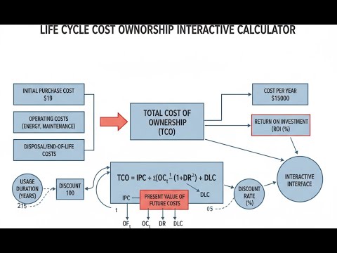
Life cycle cost (LCC) is the real sum you pay for equipment or systems from purchase to disposal. This includes everything: initial outlay, setup, ongoing energy, repairs, downtime, and removal or salvage at the end. The goal is an honest comparison of what you’ll really end up paying over the years—not just what’s on the invoice the day it arrives.

Simple Explanation

If you’ve ever owned a car, you know the cheapest one at the dealership might chew up your wallet in fuel and repair costs over ten years, compared to a pricier but more reliable vehicle. Industrial and facilities equipment work no differently—LCC takes the long view, adding up every bill you'll face, not just the first one. You're aiming for the lowest total, not just the lowest sticker price.

📐 Browse all 1000+ Interactive Calculators

Visual Diagram: Life Cycle Cost Components

Life Cycle Cost Ownership Calculator

How to Use This Calculator

1. Pick the calculation mode: Total Life Cycle Cost, NPV Analysis, Compare Two Options, Break-Even, or Annual Equivalent Cost.
2. Type in the cost numbers for your case—purchase price, installation, yearly operating/energy/maintenance/downtime, service life, discount rate, and salvage value, depending on the mode.
3. Set service life and discount rate so they match your actual expectations or company assumptions.
4. Hit Calculate. You'll get your results in a few seconds.

Formulas & Life Cycle Cost Equations

Use the formula below to calculate total life cycle cost.

Use the formula below to calculate net present value.

Use the formula below to calculate annual equivalent cost.

Use the formula below to calculate break-even period.

Simple Example

Equipment A comes in at $20,000, costs $1,000 to install, and needs $3,000/year to run (including maintenance and energy). The unit will last 5 years, and when scrapped, it's worth $500.

LCC = ($20,000 + $1,000) + ($3,000 × 5) − $500 = $21,000 + $15,000 − $500 = $35,500

Annualized cost = $35,500 ÷ 5 = $7,100/year

Theory & Engineering Applications of Life Cycle Costing

Life cycle cost analysis takes you well beyond “what’s the cheapest upfront.” What you specify in procurement will lock in decades of energy use, downtime risk, and maintenance headaches or savings. Take this compressor example: a $100,000 model with 85% efficiency, or a $140,000 option at 93%. Run them 6,000 hours a year, 75 kW load, $0.12/kWh, for 20 years, and the higher efficiency saves about $108,000 just on power—even after paying a hefty 40% more at the start. This is why LCC stops surprises later.

Time Value of Money and Discount Rate Selection

The discount rate converts future costs into their present-day equivalent. It’s not just finance-speak; it has real effect on your totals. Public infrastructure might use 3-7%, private industry often expects 10-15% (to match investor/loan requirements). Lower rates (2-4%) are used for things like military or infrastructure likely to stay around for decades, while fast-moving tech gets high rates (12-18%) because replacement is quick. For context: a $50,000 cost in 15 years is worth $32,076 at 3%, but only $11,970 at 10%. High discount rates make future costs look smaller. That’s why they tend to favor lower upfront spend—just know what your rate is actually representing.

This explains why high discount rates favor lower initial costs with higher operating expenses — future costs become heavily discounted. Defense procurement often uses lower rates (2-4%) because assets serve national security over 30-50 year horizons, while technology equipment uses higher rates (12-18%) reflecting rapid obsolescence and 3-5 year replacement cycles.

Hidden Cost Categories in Industrial Systems

Downtime is often underestimated or ignored in cost models. In fast-moving production, the dollar loss per hour can quickly eclipse anything you save on equipment. Imagine a bottling line creating $18,000/hour in value; add in labor and ruined material, and downtime's real impact can hit $25,000-$30,000 per hour. If a machine with 99.2% uptime only stops 149 hours/year, but 97.5% stops for 219 hours, that 70-hour difference at $25k/hour is a $1.75 million swing each year. This same thinking applies in auto factories, chip plants, food production—anywhere process shutdowns cause cascading effects.

At $25,000/hour, this represents $1.75 million in annual value difference, justifying substantial initial cost premiums for higher-reliability equipment. This calculation method applies across automotive assembly, semiconductor fabrication, and food processing where line stoppages cascade through integrated production systems.

Energy Cost Escalation and Long-Term Projections

If you’re in energy-intensive industries, don’t assume today’s utility rates will last. For instance, U.S. industrial electric rates have risen by almost half from 2000 to 2023—about 1.7% faster per year than inflation. Smart LCC uses an energy escalation rate above inflation (often 2-3% more per year, separate from the general discount). If you run a 2.5 MW data center and project a modest 2.5% escalation, over 15 years at $0.08/kWh baseline, you’re looking at $8.7 million in extra spend compared to flat rates. Any new drive, efficient motor, or lighting system justifies its higher initial cost more convincingly when you factor in these escalation patterns. Always break out your energy expenses and use reasonable, documented rates based on historical data.

Variable frequency drives, high-efficiency motors, heat recovery systems, and LED lighting retrofits all demonstrate enhanced economic justification when energy escalation factors enter the analysis. Process industries performing LCC analysis should separate energy costs from other operating expenses and apply sector-specific escalation rates based on fuel type — natural gas, electricity, or diesel — each following distinct price trajectories.

Worked Example: HVAC System Selection for Commercial Building

A 150,000 square foot office building in Chicago needs a new HVAC setup. Here are two choices:

Option A: Standard Efficiency System
Initial equipment cost: $385,000
Installation cost: $95,000
Annual energy consumption: 1,850,000 kWh at $0.095/kWh = $175,750/year
Annual maintenance: $18,500
Service life: 18 years
Salvage value: $12,000

Option B: High Efficiency System with Heat Recovery
Initial equipment cost: $565,000
Installation cost: $115,000
Annual energy consumption: 1,295,000 kWh at $0.095/kWh = $123,025/year
Annual maintenance: $24,750
Service life: 22 years
Salvage value: $28,000

With a 5% discount rate and 2% annual energy cost escalation, calculate NPV for 18 years (so both options get the same period):

Option A Calculations:
Initial costs: $385,000 + $95,000 = $480,000
Year 1 operating cost: $175,750 + $18,500 = $194,250
Year 2 operating cost: ($175,750 × 1.02) + $18,500 = $197,758
Continue for 18 years, discounting each year's cost (PV = Cost / (1.05)^year)

Add them up:
PV of operating costs (years 1-18): $2,847,365
PV of salvage value: $12,000 / (1.05)¹⁸ = $4,992
Total LCC (Option A): $480,000 + $2,847,365 - $4,992 = $3,322,373

Option B Calculations:
Initial costs: $565,000 + $115,000 = $680,000
Year 1 operating cost: $123,025 + $24,750 = $147,775
Year 2 operating cost: ($123,025 × 1.02) + $24,750 = $150,236
Using the same method over 18 years:
PV of operating costs (years 1-18): $2,174,483
Total LCC (Option B, 18-year analysis): $680,000 + $2,174,483 = $2,854,483

Economic Comparison:
Net savings with Option B: $3,322,373 - $2,854,483 = $467,890
Savings as percentage: 14.1% over analysis period
Simple payback period: ($680,000 - $480,000) / ($194,250 - $147,775) = 4.3 years
Discounted payback: Roughly 5.1 years (counting time value)

Despite a 41.7% higher upfront spend ($200,000 more), Option B saves almost $468,000 in today’s dollars over 18 years—mostly from energy savings. Its longer rated life (22 vs. 18 years) is extra value not even fully included here.

Maintenance Cost Modeling and Equipment Aging

Assuming future maintenance costs stay flat is rarely accurate in real plants. Most equipment gets more expensive to maintain as it ages—seals leak, bearings wear out, controls get outdated or unserviceable. Realistic models use a “bathtub curve”: early issues, stable years, then rising failures and costs with age. For example, an industrial pump may cost $4,000/year from years 3-10, but then jump 8-12% yearly in costs, maybe hitting $8,200/year by year 20. If you do flat-rate models, expect to underestimate cost by 15-22%. This means there’s a clear point where replacement is cheaper than stretching equipment to the bitter end.

A pump with $4,000 annual maintenance years 3-10 might require $4,320 in year 11, $4,666 in year 12, escalating to $8,200 by year 20. Incorporating this realistic cost progression into LCC analysis increases total costs by 15-22% compared to flat-rate models, favoring equipment replacement at optimal economic life rather than running assets to failure.

Sensitivity Analysis and Monte Carlo Simulation

LCC models use guesses for discount, energy, maintenance rates, usable life, and utilization—none are perfect, and small changes can swing results. To avoid blind spots, good practice is to run sensitivity analysis: vary each variable one at a time and see what tips the balance. If you want more robust results (especially for big-ticket items), run a Monte Carlo simulation. This means running thousands of scenarios with different assumed ranges, and seeing how wide your cost spread actually is—not just the average. Sometimes what looks like a sure bet turns into a tossup when you factor all possible outcome ranges. If risk matters, look at the worst-case and best-case, not just the average, before committing.

For those performing comparative economic analysis across multiple options, the engineering calculator library offers additional tools for payback period calculation, internal rate of return, and benefit-cost ratio analysis that complement LCC methodology.

Practical Applications

Frequently Asked Questions

Video Walkthrough - How to Use This Calculator