Availability Mtbf Interactive Calculator

If a system stops working without warning, you need to know three things right away: how often it fails, how long you’ll be waiting for repairs, and whether you’ll hit your uptime targets. These three numbers—MTBF, MTTR, and availability—are tied together by the math, so if one is off, your plans won’t match reality. The calculator below lets you solve for any of these values using your own data or a set target. It’s as practical for a mine haul truck as it is for a production line or a server farm, wherever downtime costs money. You’ll find all the main calculation options, the formulas, a worked-through example, and a FAQ aimed at real-world engineering issues.

What is Availability and MTBF?

Availability is simply the percent of time your system can actually do its job. MTBF, or Mean Time Between Failures, is the average running time you get between breakdowns. These two numbers give you a good sense of the day-to-day reliability you’ll end up dealing with.

Simple Explanation

Picture a delivery van: it breaks down once every 500 hours of use and takes 10 hours to fix. You’ll get about 98% availability. MTBF is just the typical stretch between failures. The math is straightforward—the more time between failures and the quicker you fix them, the more available your system will be.

📐 Browse all 1000+ Interactive Calculators

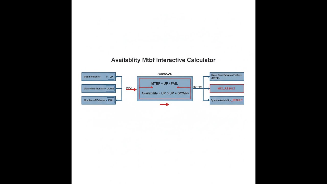
System Reliability Diagram

How to Use This Calculator

1. Pick what you want to solve for—Availability, MTBF, MTTR, Failure Rate, or something based on actual time and failure counts.
2. Fill in the required inputs for your case—hours for MTBF or MTTR, a percent for availability, or your operational numbers depending on the mode.
3. Hit "Try Example" if you want to see sample numbers worked out in real time.
4. Click Calculate to get your answer.

Simple Example

Mode: Calculate Availability from MTBF & MTTR

• MTBF = 5000 hours
• MTTR = 24 hours
• Result: A = 5000 / (5000 + 24) = 99.52% availability

Availability & MTBF Calculator

Reliability Equations

Here are the standard equations for availability, MTBF, and related values. These are what you’ll use on paper or in any calculator of this type.

Use the formula below to calculate MTBF from a known availability target and repair time.

Use the formula below to calculate maximum allowable MTTR from a target availability and known MTBF.

Use the formula below to calculate failure rate from MTBF.

Use the formula below to calculate MTBF directly from field data.

Use the formula below to calculate availability from time-tracking records.

Theory & Engineering Applications

Availability and MTBF are core to practical reliability work. They tell you, in plain terms, when your equipment is likely to be up and running, and how much downtime you’ll likely fight. These numbers matter for everything from deciding what spares to keep on hand, to justifying a maintenance budget, or arguing over equipment specs with a vendor.

The relationship between availability, MTBF, MTTR, and failure rates is what lets you set real expectations before you buy a system, or estimate the cost of making a change. You don’t need advanced statistics to make solid decisions, but you do need to know how these trade off against each other.

Fundamental Reliability Theory

Availability measures the fraction of total time the system can run. That’s just uptime divided by the whole time span. The standard formula, A = MTBF/(MTBF + MTTR), comes from the real-world pattern of operation, breakdown, and repair—round and round it goes. This approach makes sense for anything you intend to fix when it fails, rather than toss and replace. If you’re only interested in time until first failure (say, for a fuse or a light bulb), you’d use a different approach entirely (R(t) = e^-λt).

Most of the time, you’ll see reliability estimates based on a simple exponential distribution—that is, the failure rate stays constant over time, so λ = 1/MTBF. This makes the math easy, but it has a big catch: real equipment usually doesn’t behave that simply. You’ll see early failures (the “burn-in” phase), followed by a period of steady operation, then failures become more common as wear and tear increase (the “wear-out” phase). The exponential model works best during that long middle period. If you’re dealing with gear that “ages out” or shows clear signs of wear, you should be using a Weibull model instead, which gives you MTBF = η·Γ(1 + 1/β) with scale (η) and shape (β) fitted to actual data.

MTTR Components and Hidden Losses

MTTR is often misunderstood. It isn’t just turning the wrench. You have to include time to detect the failure, figure out what’s happened, order or find the parts (and wait for them), plus any admin delays, and even re-starting and testing before you’re back in business. In practice, actual downtime per event is often two to five times the pure ‘wrench time’. For example, swapping a hydraulic seal might take 3 hours on the bench, but if you count all the overhead—diagnosis, overnight parts, paperwork, and retesting—you might be facing 27 hours before the equipment is actually running. That’s why there’s a big difference between Mean Time To Repair (fixing) and Mean Time To Restore (everything from failure to green light).

Getting MTTR down is usually faster and cheaper than trying to push MTBF higher. Early fault detection tools (condition monitoring, vibration analysis, etc.) cut out a huge chunk of wasted time. If you catch problems before they snowball, you can tie repairs to planned maintenance, and keep your actual downtime per event much lower—even when your failure rate itself doesn’t change.

Series and Parallel System Configurations

For systems where every part has to work for the whole thing to run (series), total availability is the product of every component’s availability. For example, with six machines at 98% each, your line ends up at 0.98⁶ = 88.6%—a harsh drop and a real issue in complex setups. This is why you get diminishing returns as you bolt more things together; every weak link drags down the whole system.

If you can use parallel redundancy (only one unit needs to work), the math flips: A_parallel = 1 - (1 - A₁)(1 - A₂)...(1 - A_n). With two hot-standby pumps at 95% each, you reach 99.75%. In the real world, however, some problems can knock out both (like a power surge, or bad fuel). If you allow for 5% common-mode failures, true availability drops to about 99.5%. It’s important to be honest about what “independent failures” really means for your case.

Industry-Specific Availability Requirements

How much uptime you need depends entirely on how bad the consequences are. Data centers aiming for Tier IV want 99.995%—less than half an hour of downtime a year—by throwing redundancy at everything, including power and cooling. Telecom shoot for “five nines” (99.999%), getting repair times under 15 minutes through hot spares and round-the-clock teams.

Factories may be satisfied with 95–98% if running flat out, but for less critical lines (where there are production buffers), even 85–90% can be enough. In mining, where you’re limited by haul truck bottlenecks and parts can take days to arrive, 85–90% is a realistic goal for the mobile equipment.

Availability vs. Utilization Distinction

Don’t mix up availability and utilization. You might have 99% availability, but if parts or people aren’t ready, the real output could be only 60% of potential. OEE (Overall Equipment Effectiveness) is the fuller story: it combines availability, speed, and quality. Even with high availability, real process output can fall short if the other two factors aren’t managed properly.

Worked Example: Production Line Availability Analysis

Here’s a real-world calculation for a wafer fab tool running continuously. Over one quarter (2190 hours), it suffered:

• 14 unplanned breakdowns
• 127 hours total downtime (all causes included)
• 2063 hours uptime
• 18 hours preventive maintenance (counted as uptime for availability)

Step 1: Calculate actual availability from uptime/downtime

A = 2063 / (2063 + 127) = 94.20%

Step 2: Calculate MTBF from operational data

MTBF = 2190 / 14 = 156.43 hours between failures

Step 3: Calculate MTTR from downtime and failure count

MTTR = 127 / 14 = 9.07 hours per event

Step 4: Verify availability using MTBF/MTTR formula

A = 156.43 / (156.43 + 9.07) = 94.52%

The slight mismatch (94.20% vs 94.52%) is expected—the first calculation is based on raw measurement, while the MTBF/MTTR formula gives a steady-state estimate. The two converge over long periods, but don’t expect them to match exactly unless conditions are truly stable throughout.

Step 5: Determine required MTTR to achieve 96% availability target

MTTR = 156.43 × (1 - 0.96) / 0.96 = 6.52 hours

If you want to jump from current MTTR of 9.07 hours to the target 96% availability, you’ll need to shave about 2.5 hours per repair event. Not always an easy win, so pick your improvement focus carefully.

Step 6: Alternative approach — improve MTBF while holding MTTR constant

MTBF = (9.07 × 0.96) / (1 - 0.96) = 217.75 hours

If you can’t fix faster but can reduce failure frequency, you’d need to boost MTBF by roughly 39% to make the same jump in availability.

Step 7: Calculate failure rate and interpret

λ = 1 / 156.43 = 0.006392 failures per hour (~56 per year)

This is higher than what world-class fabs expect (~24–30 per year), so you’ve got improvement ground to cover. The basic tradeoff is: will it be cheaper to improve repair time, or to reduce failures through better maintenance or design?

Use these calculations as a practical tool for your maintenance, engineering, and management discussions. They’ll point you toward the most cost-effective way to improve uptime in your operation.

More calculators and reliability resources are listed in the Engineering Calculator Library, covering maintenance, reliability, and practical uptime analysis.

Practical Applications

Frequently Asked Questions

Video Walkthrough - How to Use This Calculator