Reliability Mtbf Mttr Interactive Calculator

The Reliability MTBF MTTR Interactive Calculator enables engineers, maintenance managers, and quality professionals to analyze system reliability, availability, and maintainability metrics. Understanding Mean Time Between Failures (MTBF), Mean Time To Repair (MTTR), and related reliability parameters is essential for optimizing maintenance schedules, predicting system downtime, and making data-driven decisions about equipment replacement and operational planning across manufacturing, aerospace, telecommunications, and critical infrastructure industries.

📐 Browse all free engineering calculators

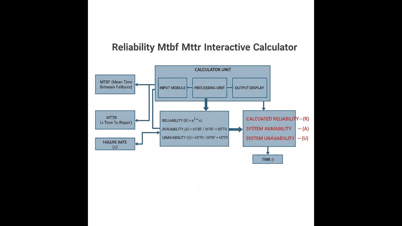
System Reliability Diagram

Reliability MTBF MTTR Calculator

Reliability Equations

Theory & Engineering Applications

Reliability engineering quantifies the probability that a system, component, or process will perform its intended function under specified conditions for a defined period. MTBF (Mean Time Between Failures) and MTTR (Mean Time To Repair) represent the two fundamental metrics that govern system availability and operational efficiency. While MTBF measures the average operational time between consecutive failures, MTTR quantifies the average time required to restore a failed system to operational status. These metrics form the foundation for predictive maintenance strategies, spare parts inventory optimization, warranty cost estimation, and life-cycle cost analysis across virtually every engineering discipline.

Understanding MTBF and Its Limitations

MTBF applies specifically to repairable systems and represents the arithmetic mean of operating time between failures. It is calculated by dividing total operating hours by the number of failures observed during that period. For a manufacturing line that operates 8,760 hours per year (continuous operation) and experiences 12 failures, the MTBF equals 730 hours. This metric assumes that failures follow an exponential distribution, which is valid during the "useful life" phase of a system's bathtub curve—after infant mortality failures have been eliminated but before wear-out mechanisms dominate.

A critical but often overlooked distinction exists between MTBF and Mean Time To Failure (MTTF). MTTF applies to non-repairable items or components that are replaced upon failure rather than repaired. For repairable systems, MTBF equals MTTF only when repair time is negligible. In practical applications, semiconductor devices use MTTF specifications because failed chips are replaced, not repaired, while industrial machinery specifications typically cite MTBF because failed motors, pumps, and actuators undergo repair and return to service.

The failure rate (λ), expressed as failures per unit time, represents the reciprocal of MTBF: λ = 1/MTBF. For the manufacturing line example with MTBF of 730 hours, the failure rate equals 0.00137 failures per hour, or 1.37 failures per 1,000 hours, or approximately 12 failures per year. Failure rate specifications vary by industry convention—aerospace typically uses failures per million hours, telecommunications uses FITs (Failures In Time, failures per billion device-hours), and automotive uses failures per thousand vehicles per year.

MTTR and Maintainability Engineering

MTTR encompasses more than just active repair time. The complete downtime cycle includes failure detection time, administrative delay (obtaining approvals, scheduling technicians), logistic delay (acquiring spare parts), active repair time, system checkout, and restoration to full operational status. In modern industrial facilities, active repair often represents only 30-40% of total MTTR, with logistics and administrative delays consuming the majority of downtime. Advanced maintenance strategies focus on reducing these non-repair components through predictive monitoring, pre-positioned spare parts inventories, and streamlined approval processes.

Organizations track multiple MTTR variants to understand different aspects of maintainability. Mean Time To Detect (MTTD) measures how quickly failures are identified—critical in distributed systems where failure notification may be delayed. Mean Time To Respond (MTTR-Response) quantifies how long until a technician begins addressing the failure. Mean Time To Restore (MTTR-Restore) includes all verification and testing before returning the system to production. The simple MTTR calculation (total repair time divided by number of repairs) provides an averaged metric, but the distribution of repair times often reveals more actionable insights than the mean alone.

Availability Analysis and System Design

System availability, defined as A = MTBF / (MTBF + MTTR), represents the proportion of time a system is operational and available for use. For the manufacturing line with MTBF of 730 hours and MTTR of 4 hours, availability equals 730 / (730 + 4) = 0.9945, or 99.45%. This seemingly impressive availability translates to approximately 48 hours of downtime per year—potentially unacceptable for continuous process industries where every hour of downtime costs hundreds of thousands of dollars in lost production and quality issues.

Availability requirements drive fundamental design decisions. Achieving "five nines" availability (99.999%, or 5.26 minutes of downtime per year) requires either extraordinarily high MTBF, extremely low MTTR, or redundant system architectures. Telecommunications infrastructure achieves five nines through N+1 redundancy, where N systems carry the load and one standby system provides immediate failover capability. Data centers employ N+2 or even 2N redundancy for mission-critical applications, effectively doubling capital costs to ensure continuous operation.

The relationship between availability, MTBF, and MTTR reveals a non-obvious design principle: beyond a certain point, reducing MTTR yields greater availability improvements than increasing MTBF. For a system with MTBF of 10,000 hours and MTTR of 100 hours (98.52% availability), doubling MTBF to 20,000 hours improves availability to 99.50%—a gain of 0.98 percentage points. However, halving MTTR to 50 hours while maintaining MTBF at 10,000 hours improves availability to 99.50%—the same improvement. Further reducing MTTR to 10 hours yields 99.90% availability. This explains why modern maintenance strategies emphasize rapid response and modular replacement over perfect reliability.

Reliability Prediction and Mission Success

The exponential reliability function R(t) = e^-t/MTBF predicts the probability that a system will operate without failure for a specified mission duration. For an unmanned aerial vehicle with MTBF of 500 hours conducting a 10-hour reconnaissance mission, the mission reliability equals e^-10/500 = e^-0.02 = 0.9802, or 98.02%. This indicates approximately a 2% probability of mission failure due to system malfunction. Military planners use these calculations to determine required redundancy levels, spare aircraft allocation, and mission risk acceptance criteria.

Reliability decreases exponentially with mission duration, creating practical limits on single-string system designs. A communication satellite with MTBF of 100,000 hours faces R(87,600 hours) = e^{-87,600/100,000} = 0.417, or only 41.7% probability of completing a 10-year mission without failure. This explains why satellites incorporate extensive redundancy: dual transponders, multiple reaction wheels, backup power systems, and redundant command processors. The system-level reliability requirement drives component-level MTBF specifications through reliability allocation and fault tree analysis.

Fully Worked Engineering Example: Industrial Compressor Analysis

Consider a pharmaceutical manufacturing facility that operates a critical air compressor system 24 hours per day, 365 days per year. Over the past two years (17,520 hours), maintenance records show 27 compressor failures with total repair time of 143.4 hours. The facility manager needs to evaluate current reliability, calculate expected downtime for the upcoming year, and assess the financial impact of potential reliability improvements. Production downtime costs $3,850 per hour due to batch losses, environmental control failures, and labor inefficiency.

Step 1: Calculate Current MTBF

MTBF = Total Operating Time / Number of Failures = 17,520 hours / 27 failures = 648.89 hours

Step 2: Calculate Current MTTR

MTTR = Total Repair Time / Number of Repairs = 143.4 hours / 27 repairs = 5.311 hours

Step 3: Calculate System Availability

A = MTBF / (MTBF + MTTR) = 648.89 / (648.89 + 5.311) = 648.89 / 654.20 = 0.9919, or 99.19%

Step 4: Calculate Failure Rate

λ = 1 / MTBF = 1 / 648.89 hours = 0.001541 failures per hour = 1.541 failures per 1,000 hours = 13.50 failures per year (8,760 hours)

Step 5: Project Annual Performance

For the upcoming year (8,760 hours):

• Expected number of failures = 8,760 hours / 648.89 hours = 13.50 failures
• Expected total repair time = 13.50 failures × 5.311 hours = 71.70 hours
• Expected downtime cost = 71.70 hours × $3,850/hour = $276,045
• Actual operational time = 8,760 - 71.70 = 8,688.3 hours (99.18% uptime)

Step 6: Evaluate Improvement Scenarios

The facility evaluates two improvement options:

Option A: Implement predictive maintenance using vibration analysis and oil monitoring (cost: $45,000), expected to improve MTBF to 950 hours (reducing failures from 13.5 to 9.22 per year):

• New expected failures = 8,760 / 950 = 9.22 per year
• New repair time = 9.22 × 5.311 = 48.97 hours
• New downtime cost = 48.97 × $3,850 = $188,535
• Annual savings = $276,045 - $188,535 = $87,510
• Payback period = $45,000 / $87,510 = 0.514 years (6.2 months)
• New availability = 950 / (950 + 5.311) = 99.44%

Option B: Invest in rapid-response maintenance with pre-positioned spare parts and dedicated technician (annual cost: $68,000), reducing MTTR from 5.311 hours to 2.0 hours while maintaining current MTBF:

• Failures remain 13.5 per year
• New repair time = 13.5 × 2.0 = 27.0 hours
• New downtime cost = 27.0 × $3,850 = $103,950
• Annual savings = $276,045 - $103,950 = $172,095
• Net benefit after costs = $172,095 - $68,000 = $104,095 per year
• New availability = 648.89 / (648.89 + 2.0) = 99.69%

Step 7: Calculate Mission Reliability

The facility must maintain sterile environment for a critical 72-hour batch process. What is the probability of completing this process without compressor failure under current conditions?

R(72 hours) = e^-72/648.89 = e^-0.1110 = 0.8949, or 89.49%

This means approximately 1 in 9 critical batch runs will experience compressor failure. Under Option A (MTBF = 950 hours):

R(72 hours) = e^-72/950 = e^-0.0758 = 0.9270, or 92.70%

Option A reduces critical batch failure risk from 10.51% to 7.30%, preventing approximately one batch loss every 3 years with associated quality investigation costs and regulatory reporting requirements.

This analysis demonstrates that Option B provides superior financial return ($104,095 annual benefit vs. $42,510 for Option A after first-year amortization), higher availability (99.69% vs. 99.44%), and faster implementation. However, Option A provides better mission reliability for critical batch processes. The final decision depends on whether the facility prioritizes overall cost reduction or reduced risk of critical batch failures with their associated regulatory complications and potential product recalls.

Advanced Reliability Concepts

Series systems exhibit reliability equal to the product of individual component reliabilities. A five-component system where each component has 98% reliability (R = 0.98) achieves system reliability of R_system = 0.98⁵ = 0.9039, or 90.39%. This rapid degradation of system reliability with component count drives the aerospace principle of "simplicity is reliability"—fewer components mean fewer failure modes. When mission requirements demand complex systems, engineers employ redundancy to counteract series reliability degradation.

Parallel redundancy dramatically improves reliability through independent backup paths. A system with two parallel components, each with reliability R, achieves system reliability R_system = 1 - (1-R)² = 1 - (failure probability)². For components with R = 0.90, parallel redundancy yields R_system = 1 - (0.10)² = 0.99, or 99% reliability—a tenfold reduction in failure probability. Triple redundancy (common in flight control systems) with R = 0.95 per channel achieves R_system = 1 - (0.05)³ = 0.999875, or 99.9875% reliability, reducing failure probability by a factor of 8,000 compared to a single channel.

The bathtub curve describes failure rate variation over a product's lifetime. During the infant mortality period, failure rate decreases as manufacturing defects manifest and are eliminated through burn-in testing and early-life quality control. The useful life period exhibits constant failure rate (the exponential distribution assumption), where failures occur randomly due to external stresses rather than aging mechanisms. The wear-out period shows increasing failure rate as fatigue, corrosion, and degradation mechanisms accumulate. MTBF calculations apply only during the constant failure rate period; time-dependent reliability models (Weibull distribution) are required for infant mortality and wear-out phases.

Practical Applications

Frequently Asked Questions