Designing optical systems, spectroscopic instruments, or quantum electronic devices requires knowing the spatial frequency of your wave — not just its temporal frequency. Use this Wavenumber Interactive Calculator to calculate angular wavenumber (k) and spectroscopic wavenumber (ν̃) using wavelength, frequency, photon energy, phase velocity, or effective mass as inputs. Accurate wavenumber values are critical in IR/Raman spectroscopy, phased array antenna design, semiconductor band structure analysis, and multilayer optical coating engineering. This page includes the fundamental equations, a worked multi-layer coating example, theory on dispersion and refractive index effects, and a full FAQ.
What is Wavenumber?
Wavenumber is the number of wave cycles — or radians of phase — that fit into one unit of distance. It is the spatial equivalent of frequency. A higher wavenumber means the wave oscillates more rapidly through space.
Simple Explanation
Think of wavenumber like the density of stripes on a barcode: the more stripes packed into a centimeter, the higher the wavenumber. When light slows down entering glass, its stripes squeeze closer together — wavenumber increases, wavelength shrinks, but the color (frequency) stays the same. Two different conventions exist: one counts full cycles per unit length, the other counts radians of phase — they differ by a factor of 2π.
📐 Browse all 1000+ Interactive Calculators
Table of Contents
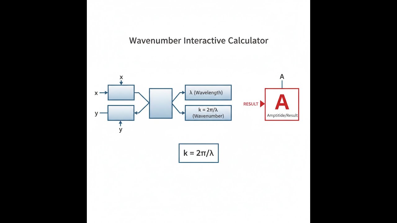
Wave Diagram

Wavenumber Interactive Calculator
How to Use This Calculator
- Select your calculation mode from the dropdown — choose from wavelength, frequency, photon energy, angular wavenumber, spectroscopic conversion, or dispersion relation.
- Enter your known values in the input fields that appear — wavelength in nm, frequency in THz or GHz, energy in eV, or wavenumber in rad/m depending on the selected mode.
- If your wave propagates through a medium other than vacuum, enter the refractive index where prompted.
- Click Calculate to see your result.
Wavenumber Interactive Visualizer
See how wavelength, frequency, and refractive index affect wave spatial frequency in real-time. Adjust the controls to visualize how waves compress when entering denser materials and how this changes the wavenumber calculation.
Angular k
1.14×10⁷
Spectroscopic ν̃
18,182 cm⁻¹
Frequency
545 THz
FIRGELLI Automations — Interactive Engineering Calculators
Fundamental Equations
Use the formula below to calculate wavenumber from wavelength, frequency, phase velocity, or energy.
Angular Wavenumber:
k = 2π/λ = 2πf/vp = ω/vp
Spectroscopic Wavenumber:
ν̃ = 1/λ
Dispersion Relation (Free Space):
ω = ck
Quantum Dispersion:
E = ℏ²k²/(2m*)
Medium with Refractive Index:
k = nk0 = 2πn/λ0
k = angular wavenumber (rad/m)
ν̃ = spectroscopic wavenumber (cm⁻¹)
λ = wavelength (m)
λ0 = vacuum wavelength (m)
f = frequency (Hz)
ω = angular frequency (rad/s) = 2πf
vp = phase velocity (m/s)
n = refractive index (dimensionless)
E = energy (J or eV)
ℏ = reduced Planck constant = 1.054571817 × 10⁻³⁴ J·s
m* = effective mass (kg)
c = speed of light in vacuum = 299,792,458 m/s
Simple Example
Green light in vacuum — wavelength = 500 nm, refractive index = 1.0:
- Angular wavenumber: k = 2π / (500 × 10⁻⁹ m) = 1.2566 × 10⁷ rad/m
- Spectroscopic wavenumber: ν̃ = 1 / (500 × 10⁻⁷ cm) = 20,000 cm⁻¹
- Frequency: f = 599.6 THz
- Photon energy: 2.480 eV
Theory & Practical Applications
Wavenumber represents the spatial frequency of a wave — the number of wave cycles per unit distance. Unlike temporal frequency which measures oscillations in time, wavenumber quantifies the spatial periodicity of wavefronts. The two standard conventions reflect different physics communities: physicists and engineers prefer the angular wavenumber k = 2π/λ measured in radians per meter because it appears naturally in wave equations and Fourier transforms, while spectroscopists use ν̃ = 1/λ in reciprocal centimeters because it directly relates to molecular energy levels through E = hcν̃.
Dispersion Relations and Phase Velocity
The fundamental relationship ω = vpk connects angular frequency to wavenumber through the phase velocity. In vacuum electromagnetic waves, this reduces to ω = ck, the linear dispersion relation where phase and group velocities are identical. Dispersive media break this degeneracy — in optical fiber at 1550 nm, silica's chromatic dispersion causes different wavelengths to propagate at different velocities, with dvp/dλ ≈ -0.02 m/s/nm. This wavelength-dependent phase velocity creates pulse broadening in telecommunications systems, limiting data rates to approximately 10 Gbit/s over 80 km of standard single-mode fiber without dispersion compensation.
Material dispersion manifests through the refractive index's frequency dependence n(ω), described by the Sellmeier equation for transparent dielectrics. In semiconductor physics, electronic band structure creates highly nonlinear dispersion relations. The parabolic band approximation E(k) = ℏ²k²/(2m*) near the Γ-point in GaAs yields an effective mass m* = 0.067me, giving k = 5.27 × 10⁷ rad/m for electrons with 100 meV kinetic energy. This corresponds to a de Broglie wavelength of 119 nm — well below optical wavelengths but resolvable in electron diffraction experiments.
Spectroscopic Applications and Energy Units
Infrared spectroscopists universally report absorption peaks in wavenumbers (cm⁻¹) rather than wavelengths because vibrational energy levels scale linearly with ν̃. The C-H stretching mode in methylene groups appears at 2850 cm⁻¹ regardless of the molecule — a wavelength of 3.509 μm. This wavenumber corresponds to a photon energy of 353.3 meV or 0.3533 eV, calculated via E(eV) = 0.00012398 × ν̃(cm⁻¹).
The convenience of this unit becomes apparent when building spectral libraries: a database storing peak positions as wavenumbers can directly compare spectra regardless of instrument configuration, whereas wavelength calibration depends on spectrometer optics and detector geometry.
Raman spectroscopy reports Stokes shifts relative to the excitation laser wavenumber. Using a 532 nm Nd:YAG laser (ν̃laser = 18,797 cm⁻¹), a diamond sample exhibits a sharp phonon peak at —ν̃ = 1332 cm⁻¹ Stokes shift, corresponding to an absolute wavenumber of 17,465 cm⁻¹ (572.5 nm scattered light). The wavenumber representation immediately reveals this corresponds to 165.2 meV phonon energy — the zone-center optical phonon energy in diamond's crystal structure.
Refractive Index Effects and Optical Path Length
When light enters a dielectric medium with refractive index n, the vacuum wavenumber k0 = 2π/λ0 increases to k = nk0 while the frequency remains constant. For a 1064 nm Nd:YAG laser entering BK7 glass (n = 1.5067 at 1064 nm), the wavelength compresses to λ = 706.2 nm inside the glass while k increases from 5.906 × 10⁶ rad/m to 8.900 × 10⁶ rad/m. This 50.7% increase in spatial frequency underlies the focusing power of lenses — the shorter wavelength allows tighter confinement approaching the diffraction limit. The optical path length Lopt = nLgeom accumulates phase Φ = kLopt, creating interference patterns in thin-film coatings and Fabry-Pérot etalons.
Group velocity dispersion (GVD) in optical systems is quantified through the second derivative d²k/dω², typically expressed in ps²/km for fiber optics. Standard SMF-28 fiber exhibits GVD = +17 ps²/km at 1550 nm, meaning a 1 ps transform-limited pulse broadens to 1.83 ps after 1 km propagation. This effect becomes critical in ultrafast laser systems where maintaining pulse duration requires dispersion pre-compensation using chirped mirrors or prism pairs that introduce negative GVD to cancel material dispersion.
Worked Example: Multi-Layer Optical Coating Design
Problem: Design a quarter-wave stack anti-reflection coating for a silicon photodetector (nSi = 3.48) operating at λ0 = 850 nm. The coating uses alternating layers of TiO2 (nH = 2.35) and SiO2 (nL = 1.46). Calculate the physical thickness and wavenumber in each layer, then determine the phase shift for light traversing one complete H-L pair.
Solution:
Part A: Calculate layer thicknesses for quarter-wave optical thickness at 850 nm.
Quarter-wave optical thickness: n·d = λ0/4
TiO2 high-index layer:
dH = λ0/(4nH) = 850 nm / (4 × 2.35) = 90.43 nm
SiO2 low-index layer:
dL = λ0/(4nL) = 850 nm / (4 × 1.46) = 145.55 nm
Part B: Calculate wavenumber in each layer.
Vacuum wavenumber:
k0 = 2π/λ0 = 2π / (850 × 10⁻⁹ m) = 7.3912 × 10⁶ rad/m
In TiO2:
kH = nH·k0 = 2.35 × 7.3912 × 10⁶ = 1.7369 × 10⁷ rad/m
λH = 2π/kH = 361.7 nm (wavelength inside TiO2)
In SiO2:
kL = nL·k0 = 1.46 × 7.3912 × 10⁶ = 1.0791 × 10⁷ rad/m
λL = 2π/kL = 582.2 nm (wavelength inside SiO2)
Part C: Calculate phase accumulation through one H-L pair.
Phase in high-index layer:
ΦH = kH·dH = 1.7369 × 10⁷ × 90.43 × 10⁻⁹ = 1.5708 rad = π/2
Phase in low-index layer:
ΦL = kL·dL = 1.0791 × 10⁷ × 145.55 × 10⁻⁹ = 1.5708 rad = π/2
Total phase through one pair:
Φtotal = ΦH + ΦL = π rad = 180°
Part D: Verify reflectance reduction at design wavelength.
For normal incidence on silicon with one H-L pair, the effective interface impedance becomes:
neff = nL²/nH = 1.46² / 2.35 = 0.907
Air-coating interface reflectance:
R1 = [(nL - 1)/(nL + 1)]² = (0.46/2.46)² = 0.0350 = 3.50%
Coating-silicon interface reflectance (reduced):
R2 = [(nSi - neff)/(nSi + neff)]² = (2.573/4.387)² = 0.344 = 34.4%
Without coating, bare silicon at 850 nm has:
Rbare = [(nSi - 1)/(nSi + 1)]² = (2.48/4.48)² = 0.306 = 30.6%
The single H-L pair increases reflectance slightly — practical AR coatings require 3-5 pairs to achieve R less than 0.5% through destructive interference between multiple reflected beams.
Part E: Calculate spectroscopic wavenumber for quality control.
Spectroscopic wavenumber at design wavelength:
ν̃ = 1/λ0 = 1/(850 × 10⁻⁷ cm) = 11,765 cm⁻¹
This value appears in ellipsometry data when measuring coating thickness — the characteristic interference pattern shows maxima/minima separated by Δν̃ = 1/(2nHdH) = 2350 cm⁻¹ for the TiO2 layer, allowing non-destructive thickness verification during production.
Antenna Arrays and Spatial Filtering
Phased array antennas use wavenumber as the spatial equivalent of temporal frequency in signal processing. A linear array with element spacing d = λ/2 creates a spatial sampling rate ks = 2π/d = 4π/λ. To avoid grating lobes (spatial aliasing), the array factor must satisfy kmax less than ks/2, limiting the maximum steering angle. For a 10 GHz radar (λ = 3 cm) with d = 1.5 cm spacing, the wavenumber in free space is k = 209.44 rad/m, while the array's spatial Nyquist limit is kNyquist = 209.44 rad/m, allowing steering to ±90° without grating lobes. Decreasing spacing to d = λ/4 increases ks to 8π/λ, enabling superdirective patterns but at the cost of mutual coupling between elements.
Quantum Mechanics and Crystal Momentum
In solid-state physics, the crystal momentum ℏk serves as a quasi-momentum for electrons in periodic lattices. Bloch's theorem restricts physically distinct states to the first Brillouin zone |k| ≤ π/a where a is the lattice constant. For silicon with a = 5.431 Å, the zone boundary occurs at kmax = 5.788 × 10⁹ rad/m. Electrons at this wavenumber have kinetic energy E = ℏ²k²/(2m*) = 11.4 eV for free-electron mass, but band structure modifications reduce this to the actual conduction band minimum at 1.12 eV. Conservation of crystal momentum ki + kphonon = kf governs indirect optical transitions in silicon, requiring phonon assistance because the valence band maximum and conduction band minimum occur at different k-points.
Measurement Techniques and Calibration
Fourier-transform infrared (FTIR) spectroscopy achieves wavenumber accuracy better than 0.01 cm⁻¹ through HeNe laser frequency reference at 15,798.0 cm⁻¹ (632.991 nm). The interferometer samples the optical path difference at intervals calibrated to the laser wavelength, directly producing spectra in wavenumber space via discrete Fourier transform. This surpasses diffraction grating monochromators where wavenumber ν̃ = (sin θin + sin θout)/(λgroove·m) depends on mechanical angle accuracy — typically limiting precision to 0.1 cm⁻¹ for 1200 lines/mm gratings at visible wavelengths.
For additional engineering calculations and wave physics tools, visit our free engineering calculator library.
Frequently Asked Questions
Free Engineering Calculators
Explore our complete library of free engineering and physics calculators.
Browse All Calculators →🔗 Explore More Free Engineering Calculators
About the Author
Robbie Dickson — Chief Engineer & Founder, FIRGELLI Automations
Robbie Dickson brings over two decades of engineering expertise to FIRGELLI Automations. With a distinguished career at Rolls-Royce, BMW, and Ford, he has deep expertise in mechanical systems, actuator technology, and precision engineering.
Need to implement these calculations?
Explore the precision-engineered motion control solutions used by top engineers.


