Weibull Analysis Failure Interactive Calculator

Predicting when a component will fail—and how many will fail within your warranty window—is one of the hardest problems in reliability engineering. Use this Weibull Analysis Failure Calculator to calculate reliability at a given time, instantaneous failure rate, mean time to failure, and more, using your shape parameter (β), scale parameter (η), and operating time. Getting these numbers right matters in aerospace, automotive, and medical device programs where a missed estimate translates directly to warranty cost overruns, unsafe products, or failed regulatory submissions. This page covers the Weibull equations, a worked bearing-life example, theory on the β parameter, and a full FAQ.

What is Weibull Analysis?

Weibull analysis is a statistical method for predicting how long products or components will last before they fail. You fit failure time data to a Weibull distribution to estimate the probability of survival at any point in time.

Simple Explanation

Think of it like a batting average for reliability — instead of predicting hits, you're predicting failures. You feed in a handful of real failure times, and the Weibull model tells you the pattern: are things failing early due to defects, randomly, or wearing out with age? Once you know the pattern, you can predict when the next failures are likely to happen across your entire product population.

📐 Browse all 1000+ Interactive Calculators

How to Use This Calculator

1. Select your calculation mode from the dropdown — choose from reliability at time t, failure rate, MTTF, time for target reliability, parameter estimation from data, or warranty return rate.
2. Enter your shape parameter (β), scale parameter (η), and operating time (t). If you have a failure-free period, enter the location parameter (γ); otherwise leave it at 0.
3. For the parameter estimation mode, paste your comma-separated failure times directly into the text field and provide an initial η estimate.
4. Click Calculate to see your result.

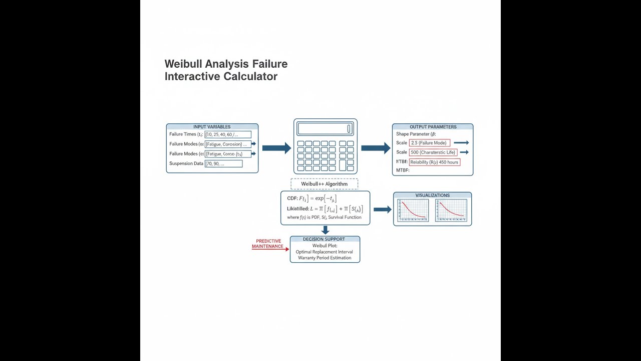
Weibull Distribution Diagram

Weibull Analysis Failure Calculator

Weibull Distribution Equations

Use the formula below to calculate Weibull reliability.

Simple Example

A bearing has β = 2.0, η = 10,000 hours, γ = 0. What is the reliability at t = 5,000 hours?

• Adjusted time: 5,000 − 0 = 5,000 hours
• Exponent: (5,000 / 10,000)² = 0.25
• R(5,000) = e^−0.25 ≈ 0.7788 → 77.88% of bearings are still running at 5,000 hours

Theory & Engineering Applications

The Weibull distribution, named after Swedish engineer Waloddi Weibull who popularized it in 1951, stands as the most versatile life distribution model in reliability engineering. Unlike the exponential distribution which assumes a constant failure rate, or the normal distribution which assumes symmetry, the Weibull distribution accommodates three fundamentally different failure behaviors through its shape parameter β: infant mortality (β < 1), random failures (β = 1), and wear-out failures (β > 1). This flexibility makes it the preferred model for analyzing everything from ball bearing fatigue to electronic component lifetimes to wind turbine blade failures.

The Shape Parameter: Window Into Failure Physics

The shape parameter β reveals the underlying failure mechanism with remarkable clarity. When β falls between 0.5 and 0.8, the decreasing failure rate indicates defect-related early failures—manufacturing defects, contamination, or assembly errors that manifest quickly. Quality control improvements and burn-in testing directly target this region. When β ranges from 2.0 to 4.5, the distribution describes mechanical wear-out: fatigue cracks in metals (β ≈ 2.0-2.5), bearing failures (β ≈ 1.5), or corrosion-induced failures (β ≈ 2.0-3.5). Values above 4.0 indicate rapid wear-out characteristic of certain polymer degradation mechanisms or severe operating stress.

The critical insight often overlooked: β is not merely a curve-fitting parameter but a diagnostic signature of the physical failure process. When β shifts unexpectedly in production data, it signals a fundamental change in failure mode—perhaps a new supplier's materials, altered manufacturing process, or different operating environment.

The Characteristic Life: More Than Just a Time Scale

The scale parameter η, called the characteristic life, represents the time at which exactly 63.2% of the population has failed (regardless of β value). This mathematical fact—derived from setting the exponent to unity—provides a shape-independent reference point. In practical terms, η serves as the natural time scale for the failure process. For rolling element bearings, η typically ranges from 10,000 to 100,000 hours depending on load and speed. For semiconductor devices, η might span from 50,000 to 500,000 hours at operating temperature.

The ratio t/η creates a dimensionless time that enables direct comparison across different products and applications. However, the characteristic life must always be interpreted alongside β: an η of 20,000 hours with β = 0.8 (infant mortality) implies very different reliability behavior than the same η with β = 3.5 (rapid wear-out).

Maximum Likelihood Estimation: The Standard for Parameter Determination

While graphical methods using Weibull probability paper provide intuitive visualization, modern reliability analysis relies on maximum likelihood estimation (MLE) for determining β and η from field or test data. MLE iteratively solves the likelihood equations to find parameter values that maximize the probability of observing the given failure data. For complete data (all units failed), the MLE equations are straightforward. For censored data—where some units have not yet failed—MLE correctly accounts for these "survivors" in the parameter estimation.

A critical practical consideration: MLE requires at least 5-10 failures for reasonable parameter estimates, with 20+ failures providing good confidence intervals. Time-censored data (test stopped at fixed time) and failure-censored data (test stopped after N failures) require different MLE formulations. The calculator's parameter estimation mode uses a simplified MLE approach suitable for complete data sets; professional reliability software handles complex censoring scenarios.

Competing Risk Analysis and Mixed Weibull Distributions

Real-world components often exhibit multiple failure modes: mechanical wear, electrical overstress, thermal degradation, and corrosion occurring simultaneously. Each mode follows its own Weibull distribution with distinct β and η values. The observed reliability is the product of individual reliabilities: R_system(t) = R₁(t) × R₂(t) × ... × R_n(t). On Weibull probability paper, this creates characteristic "dog-leg" curves where the slope changes, indicating a transition from one dominant failure mode to another.

Automotive components frequently show this behavior: early infant mortality from assembly defects (β ≈ 0.6) followed by random failures (β ≈ 1.0) from various causes, then wear-out (β ≈ 2.5) from mechanical degradation. Deconvolving these mixed distributions requires specialized software and considerable expertise, but recognizing their presence is crucial for root cause analysis.

Accelerated Life Testing and the Weibull Framework

Few products can be tested for their full design life economically. Accelerated life testing (ALT) applies elevated stress—temperature, voltage, vibration, or humidity—to induce failures more quickly. The Weibull distribution provides the statistical foundation for extrapolating from accelerated conditions to normal use. The Arrhenius model for temperature acceleration assumes β remains constant while η decreases exponentially with temperature: η(T) = A × exp(E_a/kT), where E_a is activation energy and k is Boltzmann's constant. For voltage acceleration, the inverse power law applies: η(V) = B × V^-n.

The key assumption—constant β across stress levels—must be validated experimentally; if β changes, the acceleration model may not apply, indicating different failure physics at high stress. Proper ALT design requires careful stress selection to avoid inducing unrealistic failure modes while achieving measurable failure rates within practical test durations.

Worked Example: Electric Motor Bearing Life Analysis

Consider an industrial electric motor manufacturer analyzing field return data for a 50 HP motor series. Warranty claims from 2,847 motors in service provided 73 bearing failures over 18 months. Failure times (in operating hours): ranging from 1,240 hours (earliest) to 14,780 hours (latest), with the median failure at 8,320 hours. The remaining 2,774 motors continue operating, representing right-censored data.

Step 1: Parameter Estimation
Using maximum likelihood estimation for censored data, the analysis yields:
Shape parameter: β = 2.18 (indicating wear-out failures, consistent with rolling contact fatigue)
Scale parameter: η = 18,450 hours (characteristic life)
Location parameter: γ = 0 (no failure-free period assumed)

Step 2: Calculate Key Reliability Metrics
Mean time to failure: MTTF = 18,450 × Γ(1 + 1/2.18) = 18,450 × 0.8873 = 16,370 hours
Median life (B50): t₅₀ = 18,450 × (ln 2)^1/2.18 = 18,450 × 0.8308 = 15,330 hours
B10 life (10% failure): t₁₀ = 18,450 × (-ln 0.9)^1/2.18 = 18,450 × 0.3142 = 5,797 hours

Step 3: Warranty Period Analysis
Current warranty covers 5,000 hours. Calculate expected warranty return rate:
F(5000) = 1 - exp(-[5000/18450]^2.18) = 1 - exp(-0.0725) = 1 - 0.9301 = 0.0699
Expected warranty returns: 6.99% of motors, or approximately 199 failures from 2,847 units

Step 4: Reliability at Extended Operating Time
Calculate reliability at 10,000 hours (typical inspection interval):
R(10000) = exp(-[10000/18450]^2.18) = exp(-0.3469) = 0.7070
At 10,000 hours, 70.7% of bearings remain functional, 29.3% have failed.

Step 5: Failure Rate Progression
Calculate instantaneous failure rate at 5,000, 10,000, and 15,000 hours:
λ(5000) = (2.18/18450) × (5000/18450)^1.18 = 0.000118 × 0.1876 = 2.22 × 10^-5 failures/hour
λ(10000) = (2.18/18450) × (10000/18450)^1.18 = 0.000118 × 0.4264 = 5.03 × 10^-5 failures/hour
λ(15000) = (2.18/18450) × (15000/18450)^1.18 = 0.000118 × 0.6892 = 8.13 × 10^-5 failures/hour

Engineering Decisions:
1. The β = 2.18 confirms mechanical wear-out as primary failure mode; lubrication and contamination control are critical
2. B10 life of 5,797 hours suggests current 5,000-hour warranty is aggressive; consider reducing to 4,000 hours or implementing condition monitoring
3. Increasing failure rate with time supports preventive replacement strategy; recommend bearing replacement at 12,000 hours (before failure rate accelerates significantly)
4. For high-reliability applications requiring 95% survival, limit operating time to: t = 18450 × (-ln 0.95)^1/2.18 = 18450 × 0.2235 = 4,124 hours between maintenance intervals

Confidence Intervals and Statistical Rigor

Every Weibull parameter estimate carries uncertainty inversely proportional to sample size. With 10 failures, 90% confidence bounds on β typically span from 0.5β to 2.0β; with 50 failures, this narrows to 0.75β to 1.3β. Professional reliability analysis must report confidence intervals, not just point estimates. The Fisher Information Matrix provides variance estimates for β and η, enabling construction of confidence bounds on reliability predictions.

For critical applications—aerospace, medical devices, nuclear—reliability demonstrations often require proving R(t) > R_target with 90% confidence and 90% reliability (the "90/90" criterion). This dramatically increases required test duration and sample size. The practical implication: early-stage reliability estimates from limited data should be viewed as preliminary indicators requiring validation through extended field monitoring.

For more reliability engineering tools, explore our complete calculator library, including fatigue analysis, stress-strength interference, and reliability block diagram calculators.

Practical Applications

Frequently Asked Questions