Quantifying process quality across a production run — or comparing two completely different processes on a common scale — demands a metric that normalizes defect counts against complexity. Use this Six Sigma DPMO calculator to calculate Defects Per Million Opportunities, sigma levels, and process yield using defect counts, unit totals, and opportunities per unit. It matters in manufacturing, healthcare, and financial services, where even a fraction of a sigma separates world-class from average. This page includes the core formulas, a worked example, the statistical theory behind the 1.5° shift, and a full FAQ.
What is DPMO?
DPMO stands for Defects Per Million Opportunities. It tells you how many defects would occur if your process ran one million times, adjusting for how many ways a defect could happen on each unit.
Simple Explanation
Think of it like a test score — but instead of percentage correct, you're measuring how many mistakes slip through per million chances. A higher sigma level means fewer mistakes. Six Sigma (6σ) is the gold standard: just 3.4 defects per million opportunities, which is as close to perfect as most industrial processes get.
📐 Browse all 1000+ Interactive Calculators
Visual Diagram: Six Sigma Quality Levels

How to Use This Calculator
- Select your calculation mode from the dropdown — options include converting DPMO to sigma, defects to DPMO, yield to sigma, and more.
- Enter your values into the visible input fields — defect count, units inspected, opportunities per unit, or whichever inputs your selected mode requires.
- Use the Try Example button to load a pre-filled scenario if you want to see how the calculator works before entering your own data.
- Click Calculate to see your result.
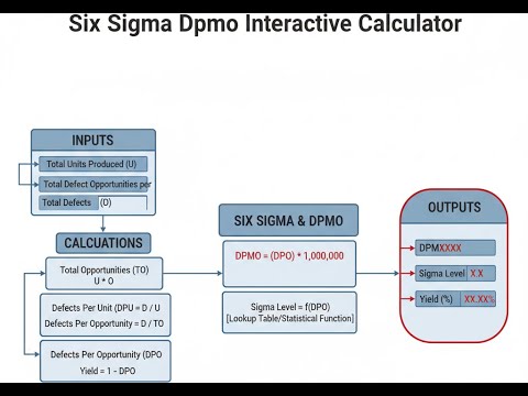
Six Sigma DPMO Interactive Calculator
Six Sigma DPMO Interactive Visualizer
Visualize how defect counts transform into sigma levels through DPMO normalization. Watch quality metrics update in real-time as you adjust defects, units, and opportunities per unit.
DPMO
1,250
SIGMA LEVEL
4.6σ
YIELD
99.88%
DEFECTS/UNIT
0.0125
FIRGELLI Automations — Interactive Engineering Calculators
Formulas & Equations
Use the formula below to calculate DPMO from raw defect data.
DPMO Calculation from Defect Data
DPMO = (D / (N × O)) × 1,000,000
Where:
- DPMO = Defects Per Million Opportunities (dimensionless)
- D = Total number of defects found (count)
- N = Number of units inspected (count)
- O = Opportunities for defects per unit (count)
Defects Per Opportunity
DPO = D / (N × O)
Where:
- DPO = Defects Per Opportunity (decimal fraction)
- D = Total number of defects (count)
- N = Number of units inspected (count)
- O = Opportunities for defects per unit (count)
Sigma Level Conversion
σ = Φ-1(1 - DPMO/1,000,000) + 1.5
Where:
- σ = Sigma level (standard deviations)
- Φ-1 = Inverse cumulative normal distribution function
- DPMO = Defects Per Million Opportunities
- 1.5 = Standard shift factor accounting for long-term process drift
Process Yield
Y = 1 - DPO = 1 - (DPMO / 1,000,000)
Where:
- Y = Process yield (fraction between 0 and 1, or percentage when multiplied by 100)
- DPO = Defects Per Opportunity
- DPMO = Defects Per Million Opportunities
Defects Per Unit
DPU = D / N = DPO × O
Where:
- DPU = Defects Per Unit (average defects found per inspected unit)
- D = Total number of defects (count)
- N = Number of units inspected (count)
- DPO = Defects Per Opportunity
- O = Opportunities for defects per unit (count)
Simple Example
A production run inspects 1,000 circuit boards. Inspectors find 10 defects. Each board has 5 opportunities for defects.
- Total opportunities = 1,000 × 5 = 5,000
- DPO = 10 / 5,000 = 0.002
- DPMO = 0.002 × 1,000,000 = 2,000
- Sigma level ≈ 4.4σ — Good, but not world class.
Theory & Engineering Applications
Fundamentals of Six Sigma Quality Metrics
Six Sigma methodology revolutionized quality management by providing a standardized language for describing process performance across vastly different industries and applications. The DPMO metric forms the cornerstone of this system, enabling direct comparison between a semiconductor fabrication process with billions of opportunities and a healthcare delivery system with hundreds. The brilliance of DPMO lies in its normalization: by expressing defects relative to opportunities rather than absolute counts, organizations can benchmark disparate processes on a common scale. A 3.4 DPMO target—equivalent to 6σ quality—represents 99.99966% defect-free performance, a level achieved by world-class manufacturers but rarely by service industries where 3σ to 4σ (66,807 to 6,210 DPMO) remains typical.
The 1.5 sigma shift embedded in the conversion formula addresses a non-obvious reality of long-term process behavior. Motorola's original Six Sigma research in the 1980s revealed that processes don't maintain perfect centering indefinitely; instead, they drift approximately 1.5 standard deviations over time due to tool wear, environmental changes, operator variation, and material batch differences. This empirical observation means that a process designed to 6σ specification limits will actually perform at 4.5σ in the long term, yielding the famous 3.4 DPMO figure. Critics argue this shift factor lacks universal applicability—highly stable automated processes may exhibit minimal drift while manual assembly operations might exceed 1.5σ—yet the convention persists because it provides conservative estimates and common ground for quality benchmarking. Engineers should recognize that the 1.5 shift is a statistical accommodation, not a physical constant, and may adjust calculations for specific process characteristics when building detailed capability studies.
Defining Defect Opportunities: The Critical Engineering Decision
Perhaps the most consequential and frequently mishandled aspect of Six Sigma analysis involves defining what constitutes an "opportunity" for defect occurrence. An opportunity must represent a discrete, measurable chance for a specific defect type to occur on a particular unit characteristic. For a printed circuit board with 847 solder joints, each joint represents one opportunity for a cold solder defect—yielding 847 opportunities per board. However, if inspecting for multiple defect types (cold solder, insufficient solder, bridging, missing component), and each joint can exhibit any defect mode, the opportunity count multiplies accordingly. Aggressive opportunity counting inflates denominators, artificially improving DPMO and sigma levels, while conservative counting produces pessimistic metrics that misrepresent true capability.
Industry consensus suggests opportunities should be countable, independent, and meaningful to the customer. A door assembly with 24 bolts doesn't have 24 opportunities if a single quality check verifies all bolts simultaneously—it has one opportunity for "improper bolt installation." Conversely, a 1200-word document checked for spelling errors has 1200 opportunities because each word represents an independent chance for error. The pharmaceutical industry exemplifies rigorous opportunity definition: a tablet manufacturing process might define opportunities as tablet weight, thickness, hardness, dissolution rate, and absence of visible defects—five opportunities per tablet. Incorrect opportunity definition can shift apparent sigma levels by a full standard deviation or more, making consistency within an organization more critical than absolute accuracy. Documentation of opportunity definitions enables valid time-series trending and meaningful process comparisons.
Statistical Foundation and Distribution Assumptions
The mathematical relationship between DPMO and sigma level relies fundamentally on the normal (Gaussian) distribution assumption for process output. When calculating sigma from DPMO, we're essentially determining how many standard deviations fit between the process mean and specification limits such that the tail area beyond specifications equals the observed defect rate. The inverse cumulative distribution function (Φ-1) converts probabilities back to z-scores, which we then adjust by the 1.5σ shift. This approach works beautifully for continuously variable characteristics (dimensions, weights, voltages) that naturally follow normal distributions due to the Central Limit Theorem's aggregation of many small independent sources of variation.
However, many real-world processes violate normality assumptions. Attribute data (pass/fail inspection results), count data (number of scratches per panel), and highly skewed distributions (wait times, chemical purity levels approaching 100%) don't conform to the bell curve. For such cases, engineers employ transformations (Box-Cox, logarithmic) to achieve approximate normality, or alternatively use non-parametric methods that estimate percentiles directly from data without distributional assumptions. Discrete manufacturing processes with multiple failure modes often exhibit bimodal or multimodal distributions that cannot be adequately characterized by a single sigma value. Advanced practitioners recognize these limitations and supplement DPMO calculations with process capability indices (Cpk, Ppk), control charts, and failure mode analysis to build comprehensive process understanding. The DPMO metric excels as a summary statistic and benchmarking tool but cannot replace detailed statistical process control for active manufacturing management.
Comprehensive Worked Example: Electronics Assembly Process
Consider a contract electronics manufacturer producing automotive engine control modules. Quality engineering has collected data from a recent production run to assess process capability and identify improvement opportunities. The scenario involves 5,247 modules inspected, with quality inspectors identifying 83 total defects across various defect categories. Each module contains 12 critical-to-quality characteristics that represent opportunities for defects: solder joint integrity on 4 major connectors, proper seating of 3 integrated circuits, correct orientation of 2 polarized capacitors, presence and torque of 2 mounting screws, and proper application of conformal coating. This yields 12 opportunities per module.
Step 1: Calculate total opportunities
Total opportunities = Units inspected × Opportunities per unit
Total opportunities = 5,247 modules × 12 opportunities/module = 62,964 opportunities
Step 2: Calculate Defects Per Opportunity (DPO)
DPO = Total defects / Total opportunities
DPO = 83 defects / 62,964 opportunities = 0.001318
Step 3: Calculate DPMO
DPMO = DPO × 1,000,000
DPMO = 0.001318 × 1,000,000 = 1,318 DPMO
Step 4: Calculate process yield
Yield = 1 - DPO = 1 - 0.001318 = 0.998682
Yield percentage = 99.8682%
Step 5: Convert DPMO to Sigma level
Using the inverse cumulative normal distribution:
Yield fraction = 0.998682
Z-score = Φ-1(0.998682) = 2.98
Sigma level = Z-score + 1.5σ shift = 2.98 + 1.5 = 4.48σ
The calculated 4.48σ performance places this process in the "good" category but below world-class 6σ targets. At 1,318 DPMO, the manufacturer can expect approximately 1.3 defects per thousand opportunities, or roughly one defect every 76 modules on average. This performance level aligns with typical automotive tier-2 supplier capabilities and meets most customer requirements, but leaves substantial room for improvement. A Six Sigma team would now Pareto-analyze the 83 defects by type, identifying that 47 defects (56.6%) involved solder joint issues, 23 defects (27.7%) were IC seating problems, and 13 defects (15.7%) were distributed across other categories. Focusing improvement efforts on soldering process controls could potentially reduce DPMO by half, moving toward 5σ performance (233 DPMO) and significantly reducing warranty costs while improving brand reputation.
Industrial Applications Across Sectors
Manufacturing industries pioneered Six Sigma adoption, with Motorola, General Electric, and Toyota achieving legendary status through rigorous application of DPMO tracking and process improvement. Modern semiconductor fabrication represents the pinnacle of Six Sigma achievement, with leading foundries maintaining better than 6σ performance (under 10 DPMO) on critical photolithography and etching processes. A single modern processor contains billions of transistors, each representing multiple defect opportunities; even 5σ performance (233 DPMO) would render most dies non-functional, necessitating the extraordinary quality levels achieved through advanced process control, real-time monitoring, and aggressive defect reduction programs. Automotive manufacturers typically target 4σ to 5σ on assembly operations, recognizing that achieving 6σ across thousands of components becomes economically impractical without automated inspection and zero-defect supply chains.
Healthcare applications of Six Sigma have grown dramatically as hospitals confront medication errors, surgical complications, and patient safety concerns. A 2006 Institute of Medicine study estimated that medication administration involves 4-5 opportunities for error per dose; at typical hospital 3σ performance (66,807 DPMO), a 300-bed facility administering 2,000 medications daily would expect 133 medication errors per day. This sobering calculation drove widespread Six Sigma adoption in healthcare, with leading institutions like Mayo Clinic and Cleveland Clinic establishing dedicated quality departments using DPMO tracking for surgical site infections, catheter-associated bloodstream infections, and patient falls. Financial services employ Six Sigma for transaction processing, credit decisions, and fraud detection, where 3.8σ performance (10,000 DPMO) in credit card processing would generate 10,000 errors per million transactions—unacceptable when processing billions of daily transactions globally. For more complex calculations and process analysis, explore the complete library of engineering calculators covering statistical methods, reliability engineering, and process optimization.
Practical Applications
Scenario: Electronics Manufacturing Quality Assessment
Jennifer, a quality manager at a consumer electronics company, needs to evaluate their smartphone assembly line performance after implementing new automated optical inspection equipment. Her team inspected 8,350 phones during the first week, finding 127 defects across 15 critical quality characteristics per phone (screen alignment, button functionality, camera focus, battery connection, etc.). Using the Six Sigma DPMO calculator in "Calculate DPMO from Defects" mode, she enters 127 defects, 8,350 units, and 15 opportunities per unit. The calculator reveals 1,014 DPMO with a sigma level of 4.58σ, representing significant improvement from their previous 3.9σ performance (12,400 DPMO). This data enables Jennifer to justify the automation investment to senior management by demonstrating quantified quality improvement and projecting reduced warranty costs of approximately $340,000 annually based on the DPMO reduction.
Scenario: Healthcare Process Improvement Initiative
Dr. Marcus Chen, leading a medication safety task force at a 450-bed regional hospital, analyzes medication administration errors as part of a Joint Commission quality improvement requirement. The pharmacy tracked 89,750 medication doses administered over one month with 347 documented errors (wrong dose, wrong time, wrong medication, or wrong patient). Each dose presents four opportunities for error, yielding 359,000 total opportunities. Using the DPMO calculator, Dr. Chen determines their current performance is 966 DPMO at 4.62σ—better than the national hospital average of 3.5σ (22,700 DPMO) but below their 5σ target. He uses the "Compare Two Processes" mode to model their improvement goal: reducing from 966 DPMO to 233 DPMO (5σ) would represent a 75.9% error reduction. This quantified target helps secure funding for barcode medication administration technology and demonstrates measurable progress toward their safety goals during subsequent quarterly reviews.
Scenario: Service Industry Benchmark Comparison
Samantha Rodriguez, operations director for a national call center handling technical support, receives quarterly quality reports showing their current defect rate is 2.3% across five quality metrics per call (accurate problem identification, correct solution provided, proper documentation, adherence to handle time, and customer satisfaction score). With 245,000 calls handled quarterly, this represents 5,635 defective interactions from 1,225,000 opportunities. She uses the calculator to convert this data: entering 5,635 defects, 245,000 units, and 5 opportunities yields 4,600 DPMO at 3.97σ. Samantha then benchmarks against their main competitor who publicly claims 4.5σ performance. Using "Calculate Metrics from Sigma Level" mode with 4.5σ input shows the competitor achieves 1,350 DPMO—70% fewer defects. This analysis provides concrete targets for her improvement roadmap, identifying that reducing defects to 1,653 total (1,350 DPMO) would match competitive performance and likely reduce customer churn by an estimated 15% based on satisfaction correlation analysis.
Frequently Asked Questions
▼ What is the difference between DPMO and DPU, and when should I use each metric?
▼ Why does the Six Sigma calculation include a 1.5 sigma shift, and is this always appropriate?
▼ How do I properly count opportunities when my product has multiple potential defect types?
▼ What sigma level should my organization target, and how do different industries compare?
▼ Can I use DPMO calculations for non-manufacturing processes like customer service or software development?
▼ How does sample size affect the reliability of my DPMO calculations, and how many units should I inspect?
Free Engineering Calculators
Explore our complete library of free engineering and physics calculators.
Browse All Calculators →🔗 Explore More Free Engineering Calculators
About the Author
Robbie Dickson — Chief Engineer & Founder, FIRGELLI Automations
Robbie Dickson brings over two decades of engineering expertise to FIRGELLI Automations. With a distinguished career at Rolls-Royce, BMW, and Ford, he has deep expertise in mechanical systems, actuator technology, and precision engineering.
Need to implement these calculations?
Explore the precision-engineered motion control solutions used by top engineers.


