If you want to know where a robotic arm’s tool will end up, you’ll need to solve the forward kinematics before you build. This 2-Link Planar Forward Kinematics Calculator gives you the X and Y position of your arm’s tip from two link lengths and two joint angles. It’s a staple for tasks like pick-and-place, SCARA arms, and educational robot projects. On this page: you’ll find the formula, a sample calculation, an engineer’s explanation, and answers to practical questions.
What is 2-Link Planar Forward Kinematics?
For a 2-link planar arm, forward kinematics just means figuring out the end-point’s X and Y coordinates if you know your two arm lengths and joint angles. There’s no shortcuts—it’s just geometry and trigonometry. Feed in your real-world measurements, out comes the position.
Simple Explanation
Picture your upper arm and forearm: you can lift your arm at the shoulder, and then bend at the elbow. Forward kinematics boils down to: if your shoulder is set to 45° and your elbow is bent 30°, where does your hand end up in space? The calculator treats each link as a vector, adds them together from the base, and pinpoints the hand’s location. That’s all there is to it.
📐 Browse all 384 free engineering calculators
2-Link Planar Manipulator System

2-Link Forward Kinematics Calculator
How to Use This Calculator
This calculator is intended for education, concept evaluation, and preliminary design. Results are based on the equations and assumptions described on this page, but cannot account for every real-world load case, tolerance, material property, environmental condition, installation detail, safety factor, code, or regulatory requirement. Verify all inputs, assumptions, units, and results independently before selecting components or using the result in a real application. Safety-critical, structural, medical, lifting, transportation, or regulated applications must be reviewed by a qualified engineer.
- Enter the length of Link 1 (L₁) — the first arm segment from the base joint.
- Enter the length of Link 2 (L₂) — the second arm segment from the elbow joint.
- Enter Joint 1 angle (θ₁) and Joint 2 angle (θ₂) in degrees. Negative values are valid — they indicate clockwise rotation.
- Click Calculate to see your result.
2-Link Planar Forward Kinematics interactive visualizer
This visualizer lets you see, step by step, how adjusting your joint angles or link lengths changes the end-effector location. You’ll get immediate feedback on X, Y, distance, and angle. It’s practical for understanding and checking what your robot arm can and can’t reach.
X POSITION
189.3 mm
Y POSITION
151.4 mm
DISTANCE
242.8 mm
END ANGLE
38.6°
FIRGELLI Automations — Interactive Engineering Calculators
Mathematical Equations
Forward Kinematics Equations
Use the formula below to calculate end-effector position for a 2-link planar manipulator.
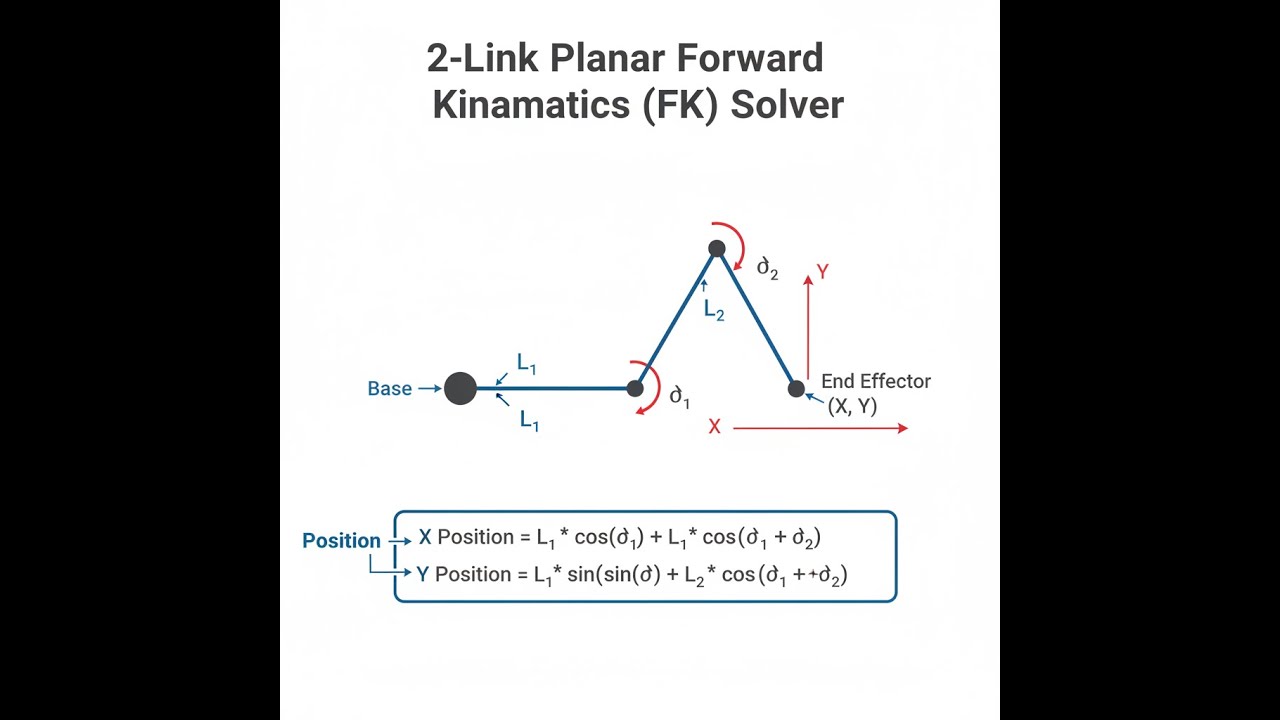
The end-effector position (X, Y) of a 2-link planar manipulator is calculated using:
Y = L₁ × sin(θ₁) + L₂ × sin(θ₁ + θ₂)
Where:
- L₁ = Length of the first link (proximal link)
- L₂ = Length of the second link (distal link)
- θ₁ = Joint angle of the first joint (base joint) measured from positive X-axis
- θ— = Joint angle of the second joint relative to the first link
- X, Y = Cartesian coordinates of the end-effector position
Additional Calculations:
End-Effector Angle: φ = atan2(Y, X)
Simple Example
L₁ = 100 mm, L₂ = 100 mm, θ₁ = 90°, θ₂ = 0°
X = 100 × cos(90°) + 100 × cos(90°) = 0 + 0 = 0 mm
Y = 100 × sin(90°) + 100 × sin(90°) = 100 + 100 = 200 mm
End-effector sits directly above the base at (0, 200 mm). Both links fully extended vertically.
Technical Guide to 2-Link Forward Kinematics
Understanding Forward Kinematics
Forward kinematics is about turning joint angles into real XY positions. In a 2-link setup, you’re adding two vectors: the first link’s reach from the base and the second link’s position from the end of the first, at a combined angle. This isn’t a complicated theory—engineers need these coordinates for anything from simple robots to test rigs.
The calculation itself is just straight geometry. The first link goes out at θ₁. The second link kicks out from the first’s tip, rotated by θ₁ + θ₂. Add those two vectors and you get your final tip location. This is what the calculator works out automatically.
Mathematical Foundation
If you want to see how the formula’s built: Each joint has a rotation and a length—it’s a coordinate transformation for each section. For a 2-link arm, the first piece points at θ₁:
- X₁ = L₁ × cos(θ₁)
- Y₁ = L₁ × sin(θ₁)
The second link starts at the end of the first and points at θ₁ + θ₂:
- ΔX₂ = L₂ × cos(θ₁ + θ₂)
- ΔY₂ = L₂ × sin(θ₁ + θ₂)
Add these up and you’ve got the end position. It’s never more complicated than the sum of those vectors.
Practical Applications
Two-link arms show up everywhere in basic automation. If you’re doing pick-and-place, small assembly, or any workspace study, you’ll be using forward kinematics to get rough or detailed locations.
Robot Programming: You need FK for path planning. If you only drive by joint angles, you never really know if the end of the arm goes where you expect. Mapping out the tip position before you run code helps avoid crashes and missed targets—especially on tasks like assembly and welding.
Workspace Analysis: FK equations tell you what area the arm can reach. Step through all joint combinations and you’ll see exactly where the end-effector can go. This helps with robot placement—no point setting up if your task is just outside the workspace.
Control System Design: Most controllers want to know X, Y for feedback. FK lets you compare where you told the robot to go (angle-wise) versus where it ended up (tip coordinates), closing the loop for real-time adjustments.
Actuator Integration: If you use FIRGELLI linear actuators instead of regular rotary motors, the same math tells you what stroke you need and where to mount things. Sometimes swapping to a linear actuator makes more sense for space or control—FK helps judge if you’ll reach your goals.
Worked Example
Let’s run the numbers for a typical arm:
- L₁ = 300 mm (first link length)
- L₂ = 200 mm (second link length)
- θ₁ = 45° (first joint angle)
- θ₂ = 30° (second joint angle)
Step 1: Get your radians:
- θ₁ = 45° × π/180 = 0.785 radians
- θ₂ = 30° × π/180 = 0.524 radians
- θ₁ + θ₂ = 1.309 radians (75°)
Step 2: Work out the X position
X = 300 × cos(0.785) + 200 × cos(1.309)
X = 300 × 0.707 + 200 × 0.259
X = 212.1 + 51.8 = 263.9 mm
Step 3: Now the Y position
Y = 300 × sin(0.785) + 200 × sin(1.309)
Y = 300 × 0.707 + 200 × 0.966
Y = 212.1 + 193.2 = 405.3 mm
This puts your tool about 264 mm across and 405 mm up from the base joint. That’s the actual, physical position, within the limits of joint accuracy and link tolerances.
Design Considerations
Singularity Avoidance: Some joint angles aren’t useful. When both links are stretched in a line (θ₂ = 0° or 180°), the arm loses flexibility—the tip can’t move in all directions. In these straight-out or folded-back positions, the robot is at a singularity. Try not to run your motion plan straight through those setups if you need full control at the tip.
Joint Limits: Physical arms always have stops, hard or soft, and sometimes odd-shaped work envelopes because of interference or hardware. Work out your real angle/window and plug that into your calculations—don’t assume you get a perfect circle just because the math says so.
Accuracy Considerations: Any errors in your arm lengths, joint misalignment, or even slight fit in the bearings will show up in the end-effector’s position. If your accuracy target is tight, calibrate the arm or run test points to see what the real world gives you. Errors stack up, especially when both links are almost collinear.
Dynamic Effects: The FK math here doesn’t factor in arm bending, vibration, or delay from actuator and software. At higher speeds or loads, you’ll see some drift from the predicted location. For slow or light-duty work, it’s a solid estimate.
Advanced Applications
Expand the basics, and you can map far more complex mechanisms. If you get comfortable with these principles, you’re equipped to move up to:
Multi-Link Extensions: Add another link, and you just keep chaining transformations—still vector and angle math, just more of it. Code gets a bit longer, but the process doesn’t fundamentally change.
3D Manipulators: For three-dimensional arms, you need extra rotation and axes (matrix transformations). Still, if your arm moves in a flat plane, the 2-link method works for that subsection of motion.
Parallel Mechanisms: Some robots have multiple arms moving a common tool. The FK for these gets trickier, but each chain is still a set of links and joints—you’ll combine their effects to get the final tip location.
Hybrid Systems: If you mix rotary and linear joints, FK lets you see how mechanical changes affect range and positioning. Using FIRGELLI linear actuators in place of some rotary axes is common when space or precision requirements dictate.
The 2-link FK method is a solid starting point for both new and experienced engineers. Whether you’re mapping out a benchtop arm, a classroom project, or looking for problems before assembly, this approach tells you what your robot can actually do—not just what it looks like on paper.
Frequently Asked Questions
📐 Explore our full library of 384 free engineering calculators →
About the Author
Robbie Dickson
Chief Engineer & Founder, FIRGELLI Automations
Robbie Dickson brings over two decades of engineering expertise to FIRGELLI Automations. With a distinguished career at Rolls-Royce, BMW, and Ford, he has deep expertise in mechanical systems, actuator technology, and precision engineering.
Need to implement these calculations?
Explore the precision-engineered motion control solutions used by top engineers.


