Darcys Law Interactive Calculator

Moving water through soil, sand, or rock comes up all the time in groundwater work, oilfields, and filter design. Get it wrong and you end up with a well that doesn't deliver, a filter that plugs, or a foundation that gets undermined. This Darcy’s Law calculator quickly gives you discharge rate, hydraulic conductivity, area, or hydraulic gradient—just pick what you need, plug in the head numbers and geometry, and go. It’s a useful tool across water projects, remediation, and reservoir work. On this page you’ll find the equations, a detailed sample calculation, the underlying theory, and a FAQ with real-world caveats.

What is Darcy's Law?

Darcy’s Law tells you how much fluid will flow through a porous material (soil, sand, rock, etc.) based on how permeable that material is, how big the cross-section is, and how much “push” you’ve got from a pressure or head difference.

Simple Explanation

Picture pushing water through a sponge. You get more water out if the sponge is bigger, wetter, or if you squeeze harder. That’s the essence of Darcy’s Law. The “hydraulic gradient” is how hard you squeeze, “hydraulic conductivity” is how easy the sponge lets water through, and “cross-sectional area” is how wide a surface you’re working with.

📐 Browse all 1000+ Interactive Calculators

How to Use This Calculator

1. Pick which variable you want to solve for—discharge rate, conductivity, area, gradient, head loss, or flow length.
2. Enter your known values (conductivity, area, head difference, length) in the fields that show up for your chosen mode.
3. If your calculation mode needs discharge rate or gradient as an input, those boxes appear—fill them in too.
4. Hit Calculate for the answer.

Simple Example

Mode: Calculate Discharge Rate (Q)

• Hydraulic Conductivity (K) = 0.0001 m/s
• Cross-Sectional Area (A) = 10 m²
• Head Difference (Δh) = 5 m
• Flow Length (L) = 100 m
• Result: Q = 0.0001 × 10 × (5/100) = 5×10⁻⁵ m³/s = 0.05 L/s

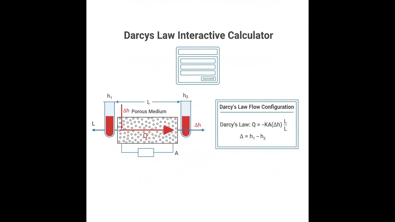
Visual Diagram

Interactive Calculator

<> Embed this calculator → <> Embed this animation calculator →

Governing Equations

These are the main formulas for getting discharge, velocity, or gradient—pick the one that matches your situation.

Theory & Practical Applications

Fundamental Physics of Darcy's Law

Darcy’s Law came out of solid experimental work on sand filters back in the 1850s and is still the go-to for describing laminar flow through soils and rock. It holds up as long as flow stays laminar—typically for Reynolds number below 1–10 in porous stuff. Unlike regular pipe flow, here you base Reynolds number on grain size, not diameter: Re = ρvd₁₀/μ (ρ is fluid density, v is Darcy velocity, d₁₀ is a typical grain size, μ is viscosity).

The hydraulic conductivity K measures how easily a fluid gets through the porous matrix. K reflects both the medium’s permeability and properties of the fluid (like viscosity and density). Permeability k (in m² or darcys) is just the material property—fluid-independent. For conversions: K = kρg/μ. For example, a sand with k = 1×10⁻¹¹ m² has K ≈ 1×10⁻⁴ m/s for water, but you can get conductivity a thousand times lower with heavy oil.

Critical Engineering Limitations and Non-Darcy Flow

Darcy’s Law is only accurate as long as you stay in linear (laminar) flow—when you start ramping up the gradient and the velocity gets high, inertial effects skew the results. In these cases, use the Forchheimer equation: i = (μ/kρg)v + (β/g)v². Once Re climbs above about 10 (in porous flow), Darcy’s Law will overpredict flow—sometimes by 15–40%. This happens most in coarse gravel, near high-rate wells, or in fractured aquifers. For fine and medium sands, you’re probably safe if Re < 1–10, but always check.

Don’t forget natural materials are rarely uniform. K can vary by factors of 100 or 1000, especially across layers. Horizontal conductivity almost always exceeds vertical in sedimentary soils. For multiple-layer aquifers, you’ll need equivalent K calculations, depending on if flow is along or across the layers.

Groundwater Engineering Applications

For wells, Darcy’s Law is the basis for estimating groundwater yield and predicting drawdown. For a fully-screened well in a confined aquifer, you use the Thiem equation, which merges Darcy’s Law with radial flow geometry. The expected well performance values in sandy aquifers can be estimated, but real-world output depends a lot on construction and geology—well efficiency and the aquifer boundaries matter.

Darcy velocity is all you get from basic analysis, but for tracking contamination, you must actually use the seepage or pore velocity: actual groundwater movement is v/n_e (Darcy velocity divided by effective porosity). For example, a contaminant in sand may move only 6 m/year even though Darcy velocities might look high. Dispersion and sorption will slow real plumes even further—if solving real problems, you need more than just Darcy’s Law.

Geotechnical and Foundation Engineering

Uplift pressures from seepage beneath dams, levees, and other structures can cause piping or heave. Analysis starts with Darcy, then turns into flow nets or numerical models for safety margins. For loose sand, critical hydraulic gradient (to avoid piping) is around 1; for design, keep actual gradients much lower using factors of safety between 2 and 4.

Settlement in soft soils, especially clays, is driven by slow drainage—Terzaghi’s consolidation is just Darcy’s Law plus how compressible your soil is. You can wait decades for thick clay layers to finish consolidating beneath a loaded building, so staged construction, surcharging, or vertical drains are routine if you want to build on a reasonable schedule.

Industrial Filtration and Petroleum Engineering

Sand or media filters, bed reactors, and similar systems are sized using Darcy’s Law for clean-bed head loss. The Kozeny-Carman equation is used if you want a better head loss estimate, especially once the filter starts clogging—effective porosity drops fast. Typical practice triggers backwashing based not just on time, but on rising head loss across the filter.

Oil and gas recovery starts with Darcy’s Law, but the story gets complicated when oil, gas, and water flow together—relative permeability drops quickly with residual fluids. Most real calculations call for numerical modeling and lab core data. Only a fraction of oil initially in place can ever be produced, and how it changes hinges on both rock and fluid properties.

Worked Example: Municipal Well Field Design

Problem: A municipality needs to design a well field in a confined sand aquifer to supply 450 m³/day (5.21 L/s) for a new residential development. Site investigation reveals the aquifer has the following properties: saturated thickness b = 18.5 m, horizontal hydraulic conductivity K_h = 3.4×10⁻⁴ m/s, vertical hydraulic conductivity K_v = 8.2×10⁻⁵ m/s, regional hydraulic gradient i₀ = 0.0018 (to the east), porosity n = 0.34, and effective porosity n_e = 0.29. The wellfield will consist of two wells spaced 85 m apart, each screened across the full aquifer thickness with 250 mm diameter screens.

Part A: Calculate the natural (undisturbed) groundwater discharge per unit width through the aquifer cross-section perpendicular to flow.

Part B: Determine the required drawdown at each well to achieve the target combined discharge of 450 m³/day, assuming both wells operate identically.

Part C: Calculate the natural seepage velocity and estimate time for a conservative tracer released 500 m upgradient to reach the well field.

Part D: Assess whether flow conditions satisfy Darcy's Law assumptions.

Solution Part A: For natural regional flow, apply Darcy's Law with the horizontal conductivity. Considering a 1 m wide cross-section perpendicular to flow:

Q_natural = K_h × A × i₀
A = b × (unit width) = 18.5 m × 1 m = 18.5 m²
Q_natural = (3.4×10⁻⁴ m/s) × (18.5 m²) × (0.0018)
Q_natural = 1.132×10⁻⁵ m³/s = 0.01132 L/s per meter width
Q_natural = 978 m³/day per meter width

This represents the natural through-flow capacity of the aquifer, which is substantial relative to the proposed pumping rate.

Solution Part B: For a fully penetrating well in a confined aquifer with radius of influence R and drawdown s at the well face (radius r_w = 0.125 m for 250 mm screen), the Thiem equation modified from radial Darcy flow gives:

Q_well = (2πKb × s) / ln(R/r_w)

Each well must produce Q_well = 450/(2 × 86400) = 2.604×10⁻³ m³/s. Assuming radius of influence R ≈ 300 m (typical for confined aquifer pumping tests, verified through type curve analysis):

2.604×10⁻³ = (2π × 3.4×10⁻⁴ × 18.5 × s) / ln(300/0.125)
2.604×10⁻³ = (0.03952 × s) / 7.886
2.604×10⁻³ = 0.005012 × s
s = 0.519 m

Required drawdown at each well face is approximately 0.52 m, which is quite modest (only 2.8% of aquifer thickness), indicating sustainable operation well within aquifer capacity. However, well interference must be checked since wells are only 85 m apart. Using principle of superposition, the total drawdown at Well 1 includes drawdown from its own pumping plus drawdown induced by Well 2 pumping 85 m away:

s_additional = Q_well × ln(R/r_separation) / (2πKb)
s_additional = 2.604×10⁻³ × ln(300/85) / (2π × 3.4×10⁻⁴ × 18.5)
s_additional = 2.604×10⁻³ × 1.258 / 0.03952
s_additional = 0.083 m

Total drawdown at each well = 0.519 + 0.083 = 0.602 m, still acceptably low.

Solution Part C: Natural seepage velocity (actual pore velocity) determines conservative tracer migration:

Darcy velocity: v = K_h × i₀ = 3.4×10⁻⁴ × 0.0018 = 6.12×10⁻⁷ m/s
Seepage velocity: v_s = v / n_e = 6.12×10⁻⁷ / 0.29 = 2.11×10⁻⁶ m/s
v_s = 0.182 m/day = 66.5 m/year

Travel time over 500 m distance (assuming purely advective transport):

t = distance / v_s = 500 m / (2.11×10⁻⁶ m/s)
t = 2.37×10⁸ seconds = 2740 days = 7.5 years

Actual breakthrough would occur earlier due to hydrodynamic dispersion and slightly faster due to well capture zone acceleration of flow, but this provides conservative estimate for wellhead protection zone delineation.

Solution Part D: Verify Darcy's Law validity by calculating Reynolds number near the well face where velocity is highest:

Maximum Darcy velocity (radial flow at well screen): v_max = Q_well / (2πr_wb)
v_max = 2.604×10⁻³ / (2π × 0.125 × 18.5) = 1.792×10⁻⁴ m/s

Using characteristic grain size d₁₀ ≈ 0.15 mm (typical for medium sand) and water properties at 15°C (ρ = 999 kg/m³, μ = 1.14×10⁻³ Pa·s):

Re = ρ × v_max × d₁₀ / μ
Re = (999 × 1.792×10⁻⁴ × 0.00015) / 1.14×10⁻³
Re = 0.0236

Since Re < 1, flow remains firmly in the laminar regime where Darcy's Law is valid, even immediately adjacent to the well screen where velocities are maximum. The design is hydraulically sound.

Frequently Asked Questions

Video Walkthrough - How to Use This Calculator