Capital equipment costs don't stay fixed — a $50,000 piece of machinery from 2005 isn't a $50,000 decision today. Inflation erodes purchasing power every year, and over a 20-30 year project lifecycle that compounding effect becomes the difference between an accurate budget and a catastrophic shortfall. Use this Inflation Adjusted Value Calculator to calculate equivalent purchasing power across time periods using original value, inflation rate, and number of years. It's directly applicable to capital equipment planning, lifecycle cost analysis, and long-term contract negotiations. This page includes the core formulas, a worked industrial example, inflation theory, and a practical FAQ.
What is Inflation Adjustment?
Inflation adjustment converts a dollar amount from one point in time into its equivalent value at another point in time, accounting for how prices rise over the years. It tells you what something would cost today — or what it would have cost in the past — if you factor in how much purchasing power has changed.
Simple Explanation
Think of it like this: a coffee that cost $1 in 1990 might cost $3 today — not because the coffee changed, but because each dollar buys less than it used to. Inflation adjustment does the same math for equipment, salaries, or any cost — it scales the number so you're always comparing apples to apples, no matter what year the price tag is from.
📐 Browse all 1000+ Interactive Calculators
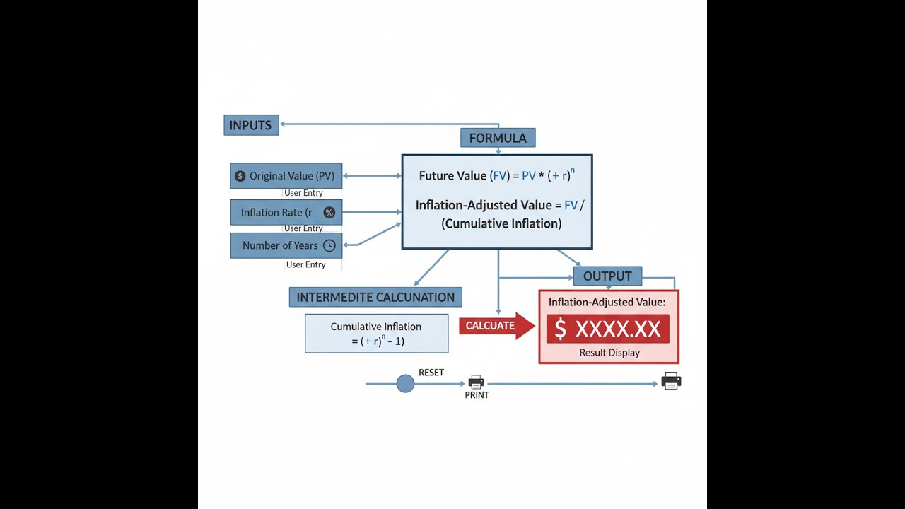
Diagram

Inflation Adjusted Value Calculator
How to Use This Calculator
- Select your Calculation Mode from the dropdown — choose whether you're solving for future value, past value, required inflation rate, time period, real return, or purchasing power loss.
- Enter the Original Value in dollars — this is the base amount you're adjusting from.
- Enter the Annual Inflation Rate (%) and Time Period (years) relevant to your scenario. If you selected Real Return mode, also enter the Nominal Return Rate (%).
- Click Calculate to see your result.
Inflation Adjusted Value Interactive Visualizer
Watch how compound inflation dramatically transforms purchasing power over time. Adjust the original value, inflation rate, and time period to see real-time calculations of future costs and cumulative inflation factors.
FUTURE VALUE
$80,050
INFLATION FACTOR
1.601×
TOTAL INCREASE
60.1%
FIRGELLI Automations — Interactive Engineering Calculators
Equations
Use the formula below to calculate inflation-adjusted value.
Future Value (Forward Inflation Adjustment)
FV = PV × (1 + r)n
FV = Future value (inflated dollars)
PV = Present value (original dollars)
r = Annual inflation rate (decimal)
n = Number of years
Past Value (Backward Inflation Adjustment)
PV = FV / (1 + r)n
PV = Past value (equivalent purchasing power in earlier period)
FV = Future/current value (today's dollars)
r = Annual inflation rate (decimal)
n = Number of years between periods
Required Inflation Rate
r = (FV / PV)1/n - 1
r = Implied annual inflation rate (decimal)
FV = Final value
PV = Initial value
n = Number of years
Time Period Required
n = ln(FV / PV) / ln(1 + r)
n = Number of years required
ln = Natural logarithm
FV = Target future value
PV = Starting present value
r = Annual inflation rate (decimal)
Real Rate of Return (Fisher Equation)
rreal = [(1 + rnominal) / (1 + rinflation)] - 1
rreal = Real rate of return adjusted for inflation (decimal)
rnominal = Nominal rate of return (decimal)
rinflation = Inflation rate (decimal)
Cumulative Inflation Factor
IF = (1 + r)n
IF = Inflation factor (multiplier for price increase)
r = Annual inflation rate (decimal)
n = Number of years
Simple Example
A piece of industrial equipment costs $10,000 today. At 3% annual inflation over 10 years:
FV = $10,000 × (1 + 0.03)10 = $10,000 × 1.3439 = $13,439
That same equipment will cost roughly $13,440 in 10 years. Budget accordingly.
Theory & Engineering Applications
Inflation adjustment calculations form the mathematical foundation for engineering economics, capital budgeting, and lifecycle cost analysis across all industrial sectors. The compound nature of inflation—where each year's increase builds upon previous years—creates exponential growth that dramatically impacts long-term financial planning. For engineering projects with 20-30 year operational horizons, failure to account for inflation can result in catastrophic underestimation of replacement costs, maintenance budgets, and total ownership expenses.
Compound Interest Mathematics and Exponential Growth
The fundamental inflation formula FV = PV × (1 + r)ⁿ represents continuous compound growth, identical in mathematical structure to radioactive decay, population growth, and chemical reaction kinetics. This exponential relationship means doubling times remain constant regardless of initial value—the Rule of 72 approximation (years to double ≈ 72/inflation rate) provides quick mental estimates. At 3% inflation, purchasing power halves every 24 years; at 6%, every 12 years. Engineers must internalize that linear thinking catastrophically underestimates long-term inflation impact: 3% annual inflation over 30 years produces not 90% cumulative inflation but 142.7% increase (2.427× multiplier).
The logarithmic inverse formulas for solving rate and time emerge from algebraic manipulation of the exponential form. Taking natural logarithms of both sides transforms the exponential equation into linear form, enabling isolation of exponent terms. This mathematical relationship explains why inflation calculators can solve for any unknown given three knowns—the system has four interdependent variables related through a single exponential equation. Understanding this mathematical unity helps engineers recognize that inflation analysis, present value discounting, and investment return calculations all share identical mathematical structures with different variable interpretations.
Real Versus Nominal Values: The Fisher Equation
The Fisher Equation distinguishes between nominal returns (raw percentage gains) and real returns (purchasing power gains after inflation). A critical non-obvious insight: the exact relationship is multiplicative, not additive. The approximation r_real ≈ r_nominal - r_inflation works only for low inflation rates; the precise formula r_real = [(1 + r_nominal)/(1 + r_inflation)] - 1 becomes essential when either rate exceeds 5%. At 8% nominal return with 3% inflation, the approximation yields 5% real return, but the exact calculation gives 4.854%—a 0.146% error that compounds significantly over decades.
This distinction matters profoundly in engineering capital allocation decisions. A manufacturing facility expansion financed at 6% interest with 2% projected inflation has a real financing cost of 3.922%, not 4%. Over a $10 million 20-year project, this 0.078% difference equals $178,000 in present value terms. Defense contractors, infrastructure projects, and energy facilities with multi-decade timelines must use exact Fisher calculations to avoid systematic budgeting errors that accumulate to millions of dollars.
Historical Inflation Variability and Predictive Limitations
A fundamental limitation engineers often overlook: inflation rates vary dramatically across sectors, commodities, and geographic regions. The US Consumer Price Index (CPI) averaged 3.28% from 1913-2023, but industrial equipment inflation, medical costs, and education expenses frequently deviate by 2-5 percentage points from general CPI. Copper prices inflated 4.1% annually 1900-2020, while computing power deflated at 30-50% annually for four decades (Moore's Law). Using aggregate inflation rates for sector-specific cost projections introduces systematic error.
Engineering cost estimation must therefore employ commodity-specific indices rather than general CPI. The Producer Price Index (PPI) for industrial machinery, Engineering News-Record Construction Cost Index (CCI), and sector-specific deflators provide more accurate projections for capital equipment, construction projects, and infrastructure development. A chemical plant expansion estimated using 3% CPI inflation versus 4.7% PPI chemical equipment inflation will underestimate 20-year replacement costs by 27.3%—potentially tens of millions of dollars on $100M+ facilities.
Lifecycle Cost Analysis and Net Present Value
Inflation adjustment integrates with discounted cash flow analysis through dual adjustments: future costs must be inflated forward, then discounted back to present value using the time value of money. The combined effect uses the real discount rate rather than nominal rate, simplifying calculations. If nominal discount rate is 8% and inflation 3%, the real discount rate of 4.854% can be applied directly to constant-dollar (inflation-adjusted) cash flows without separate inflation adjustments at each time step.
This methodology enables apples-to-apples comparison of equipment alternatives with different operational lifetimes, maintenance schedules, and replacement intervals. Comparing a $150,000 system with 15-year life versus a $225,000 system with 25-year life requires inflating future replacement costs, then discounting to present value. The first system requires replacement in year 15 at inflated cost, while the second operates 10 additional years avoiding that replacement expense. Proper inflation-adjusted NPV analysis often reverses naive initial-cost-only decisions, revealing that higher upfront investment in longer-lived equipment provides superior lifecycle value.
Worked Example: Industrial Robot Replacement Planning
A automotive manufacturing facility purchased six-axis industrial robots in 2004 for $87,500 each (installed cost). The facility plans equipment replacement in 2024 and needs to budget for equivalent modern robots. Historical data shows industrial robot prices inflated at 2.3% annually from 2004-2024, while the general CPI increased 2.6% annually over the same period. The plant operates 18 robots requiring coordinated replacement.
Step 1: Calculate time period
n = 2024 - 2004 = 20 years
Step 2: Calculate inflation factor for industrial robots
IF = (1 + 0.023)²⁰ = (1.023)²⁰ = 1.5736
Step 3: Calculate 2024 equivalent cost per robot
FV = $87,500 × 1.5736 = $137,690 per robot
Step 4: Calculate total fleet replacement budget
Total budget = $137,690 × 18 robots = $2,478,420
Step 5: Compare to CPI-based estimate
CPI inflation factor = (1.026)²⁰ = 1.6755
CPI-based estimate = $87,500 × 1.6755 = $146,606 per robot
CPI-based total = $146,606 × 18 = $2,638,908
Step 6: Calculate estimation error
Overestimation = $2,638,908 - $2,478,420 = $160,488
Percentage error = ($160,488 / $2,478,420) × 100% = 6.48%
Analysis: Using general CPI inflation (2.6%) instead of sector-specific PPI industrial equipment inflation (2.3%) would have caused the facility to overbudget by $160,488—enough to purchase an additional robot with advanced collaborative safety features. This example demonstrates why engineering cost estimation demands commodity-specific inflation data rather than economy-wide averages. The 0.3% annual inflation difference seems trivial, but compounds to 6.48% error over 20 years, representing significant capital misallocation in large-scale industrial planning.
Further calculation for lifecycle analysis: If the facility expects robots to last another 15 years before 2039 replacement, we can project forward:
2039 replacement cost = $137,690 × (1.023)¹⁵ = $137,690 × 1.4063 = $193,696 per robot
Total 2039 fleet replacement = $193,696 × 18 = $3,486,528
To establish a replacement reserve fund with annual deposits earning 5.5% nominal return (2.5% real return after 3% general inflation), we calculate the future value annuity payment:
FV = PMT × [(1 + i)ⁿ - 1] / i
$3,486,528 = PMT × [(1.055)¹⁵ - 1] / 0.055
$3,486,528 = PMT × 23.1239
PMT = $150,787 annual deposit
This comprehensive analysis shows how inflation adjustment integrates with time-value-of-money calculations to enable realistic long-term capital planning for engineering facilities. For more engineering economics tools, visit the engineering calculator hub.
Practical Applications
Scenario: Municipal Infrastructure Bond Planning
Rebecca, a civil engineer with a mid-sized city's public works department, is preparing a 30-year bond proposal to replace aging water treatment facilities. Historical records show the original 1994 treatment plant cost $14.2 million. She uses the inflation calculator with the EPA's water infrastructure cost index (4.1% annual average) to project 2024 equivalent cost: $14.2M × (1.041)³⁰ = $47.8 million. This inflation-adjusted baseline helps her justify the bond amount to city council, demonstrating that the proposed $52 million budget reflects only $4.2 million in scope expansion beyond inflation-adjusted replacement. Without this analysis, council members comparing raw 1994 versus 2024 costs would perceive a misleading 266% increase rather than the inflation-adjusted 8.8% real cost growth, potentially rejecting necessary infrastructure investment.
Scenario: Aerospace Career Salary Negotiation
Marcus, a senior aerospace engineer considering a job offer, wants to compare his current $127,000 salary with his starting salary of $68,500 from 2009 to understand real career progression. Using the calculator with 15 years and 2.4% average inflation (CPI 2009-2024), he finds his starting salary equals $96,820 in 2024 dollars. His current salary represents $30,180 real purchasing power gain—a 31.2% real increase over 15 years, or 1.84% average annual real growth after inflation. This analysis reveals his compensation has slightly lagged industry standards (2.5-3.0% real annual growth for experienced aerospace engineers), providing quantitative justification for requesting $138,000 in his new position to achieve market-rate real compensation growth. The inflation adjustment transforms vague salary comparison into concrete negotiation leverage backed by purchasing power mathematics.
Scenario: Pharmaceutical Manufacturing Equipment Replacement Reserve
Dr. Aisha Chen, facilities planning manager for a pharmaceutical production facility, manages a capital equipment replacement reserve fund for cleanroom HVAC systems currently valued at $3.8 million. The systems have 12-year design life with replacement due in 2036. She uses the calculator's real return mode to determine if the reserve fund's 6.2% nominal investment return provides adequate growth against 2.8% general inflation and 3.7% pharmaceutical equipment-specific inflation. The calculator reveals 2.35% real return after general inflation but only 1.43% real return against equipment-specific inflation. At this growth rate, the $3.8M fund will reach only $4.39M in 2036, while inflation-adjusted replacement cost will be $5.86M—a $1.47M shortfall (25% underfunded). This analysis prompts immediate action: increasing annual contributions by $97,300 or seeking higher-yield investments to close the funding gap before the replacement deadline, preventing future operational disruption or emergency budget reallocation.
Frequently Asked Questions
▼ What's the difference between nominal and real inflation-adjusted values?
▼ Should I use CPI or sector-specific inflation rates for engineering cost estimation?
▼ How do I account for inflation in international projects with multiple currencies?
▼ Why doesn't my investment return equal the inflation-adjusted result when I subtract inflation from nominal return?
▼ How far into the future can I reliably project inflation-adjusted costs?
▼ What inflation rate should I use for salary and labor cost projections in engineering workforce planning?
Free Engineering Calculators
Explore our complete library of free engineering and physics calculators.
Browse All Calculators →🔗 Explore More Free Engineering Calculators
About the Author
Robbie Dickson — Chief Engineer & Founder, FIRGELLI Automations
Robbie Dickson brings over two decades of engineering expertise to FIRGELLI Automations. With a distinguished career at Rolls-Royce, BMW, and Ford, he has deep expertise in mechanical systems, actuator technology, and precision engineering.
Need to implement these calculations?
Explore the precision-engineered motion control solutions used by top engineers.


