2-Link Planar Forward Kinematics (FK) Solver

Designing a robotic arm means knowing exactly where your end-effector will land — and that requires solving the forward kinematics problem before you build anything. Use this 2-Link Planar Forward Kinematics Calculator to calculate end-effector X and Y position using 2 link lengths and 2 joint angles. It's essential for industrial pick-and-place systems, SCARA robot design, and educational robotics platforms. This page includes the full FK formula, a worked example, a plain-English explanation, and answers to common questions.

What is 2-Link Planar Forward Kinematics?

2-link planar forward kinematics is the process of calculating where the tip of a 2-joint robotic arm ends up, given the length of each arm segment and the angle of each joint. You put in the geometry, you get out a position.

Simple Explanation

Think of your own arm: your upper arm rotates at the shoulder, and your forearm rotates at the elbow. Forward kinematics is just answering the question — if your shoulder is at 45° and your elbow is bent 30°, where is your hand? The calculator does that math instantly, treating each link as a vector and adding them together to find the final tip position.

📐 Browse all 384 free engineering calculators

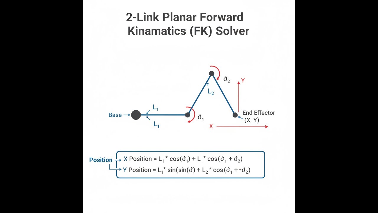
2-Link Planar Manipulator System

2-Link Forward Kinematics Calculator

How to Use This Calculator

1. Enter the length of Link 1 (L₁) — the first arm segment from the base joint.
2. Enter the length of Link 2 (L₂) — the second arm segment from the elbow joint.
3. Enter Joint 1 angle (θ₁) and Joint 2 angle (θ₂) in degrees. Negative values are valid — they indicate clockwise rotation.
4. Click Calculate to see your result.

Mathematical Equations

Simple Example

L₁ = 100 mm, L₂ = 100 mm, θ₁ = 90°, θ₂ = 0°
X = 100 × cos(90°) + 100 × cos(90°) = 0 + 0 = 0 mm
Y = 100 × sin(90°) + 100 × sin(90°) = 100 + 100 = 200 mm
End-effector sits directly above the base at (0, 200 mm). Both links fully extended vertically.

Technical Guide to 2-Link Forward Kinematics

Understanding Forward Kinematics

Forward kinematics is the process of determining the position and orientation of a robot's end-effector given the joint parameters. For a 2-link planar manipulator, this means calculating the X and Y coordinates of the end-effector based on the lengths of two links and their respective joint angles. This 2-link forward kinematics calculator serves as a fundamental tool for robotics engineers working with planar manipulator systems.

The forward kinematics problem is geometrically straightforward but computationally essential. Each link in the kinematic chain contributes to the final position through vector addition. The first link extends from the base at angle θ₁, while the second link extends from the end of the first link at angle (θ₁ + θ₂), creating a compound transformation.

Mathematical Foundation

The derivation of the forward kinematics equations begins with coordinate transformation principles. Starting from the base coordinate frame, each link represents a homogeneous transformation that includes both rotation and translation components. For a 2-link system:

The position of the first joint (end of link 1) is simply:

• X₁ = L₁ × cos(θ₁)
• Y₁ = L₁ × sin(θ₁)

The second link extends from this position at an absolute angle of (θ₁ + θ₂), contributing additional displacement:

• ΔX₂ = L₂ × cos(θ₁ + θ₂)
• ΔY₂ = L₂ × sin(θ₁ + θ₂)

The final end-effector position is the vector sum of these components, resulting in the fundamental equations used in our 2-link forward kinematics calculator.

Practical Applications

Two-link manipulator systems are ubiquitous in industrial automation, from simple pick-and-place operations to complex assembly tasks. Understanding forward kinematics is crucial for:

Robot Programming: Path planning algorithms require precise knowledge of end-effector positions. Engineers use forward kinematics to verify that programmed joint trajectories achieve desired Cartesian paths. This is particularly important when programming robots for precision assembly or welding operations.

Workspace Analysis: The forward kinematics equations define the manipulator's reachable workspace. By varying joint angles through their full ranges, engineers can map the complete set of positions the end-effector can reach, identifying optimal robot placement for specific tasks.

Control System Design: Modern robot controllers often operate in Cartesian space while commanding joint-space actuators. Forward kinematics provides the essential link between joint positions and end-effector locations, enabling real-time feedback control systems.

Actuator Integration: When designing robotic systems with FIRGELLI linear actuators, forward kinematics helps determine the required actuator stroke lengths and mounting configurations. Linear actuators can replace traditional rotary joints in certain applications, providing precise linear motion with simplified control.

Worked Example

Consider a 2-link manipulator with the following specifications:

• L₁ = 300 mm (first link length)
• L₂ = 200 mm (second link length)
• θ₁ = 45° (first joint angle)
• θ₂ = 30° (second joint angle)

Using our forward kinematics equations:

Step 1: Convert angles to radians

• θ₁ = 45° × π/180 = 0.785 radians
• θ₂ = 30° × π/180 = 0.524 radians
• θ₁ + θ₂ = 1.309 radians (75°)

Step 2: Calculate X position

X = 300 × cos(0.785) + 200 × cos(1.309)
X = 300 × 0.707 + 200 × 0.259
X = 212.1 + 51.8 = 263.9 mm

Step 3: Calculate Y position

Y = 300 × sin(0.785) + 200 × sin(1.309)
Y = 300 × 0.707 + 200 × 0.966
Y = 212.1 + 193.2 = 405.3 mm

The end-effector position is (263.9, 405.3) mm from the base origin. This example demonstrates the precision achievable with the 2-link forward kinematics calculator for practical engineering applications.

Design Considerations

Singularity Avoidance: Certain joint configurations create kinematic singularities where the manipulator loses degrees of freedom. For a 2-link arm, this occurs when both links are fully extended (θ₂ = 0°) or completely folded (θ₂ = 180°). Designers must consider these constraints when defining workspace requirements.

Joint Limits: Real manipulators have physical joint limits that constrain the theoretical workspace. Mechanical stops, actuator limitations, and collision avoidance requirements all reduce the practically achievable positions. Forward kinematics analysis must incorporate these constraints for realistic system design.

Accuracy Considerations: Manufacturing tolerances in link lengths and joint positioning affect end-effector accuracy. Error propagation through the kinematic chain can amplify small joint errors, particularly when links are nearly aligned. Precision applications may require calibration procedures to compensate for these effects.

Dynamic Effects: While forward kinematics assumes quasi-static conditions, high-speed motions introduce dynamic effects that can affect accuracy. Link flexibility, actuator dynamics, and control system bandwidth all influence the relationship between commanded and actual positions.

Advanced Applications

Modern robotic systems often extend basic 2-link concepts to more complex configurations. Understanding forward kinematics principles enables engineers to tackle:

Multi-Link Extensions: Adding additional links follows the same transformation principles, with each link contributing its own coordinate transformation. The computational complexity increases, but the fundamental vector addition approach remains valid.

3D Manipulators: Extending to three-dimensional space requires consideration of additional rotation axes and more complex transformation matrices. However, many 3D manipulators include planar subsections analyzable using 2-link techniques.

Parallel Mechanisms: Some robotic systems use parallel kinematic chains where multiple 2-link mechanisms work together to control end-effector position. Forward kinematics becomes more complex but remains based on the same fundamental principles.

Hybrid Systems: Combining rotary joints with linear actuators creates hybrid kinematic chains. FIRGELLI linear actuators can replace rotary joints in certain applications, simplifying control while maintaining precise positioning capabilities.

The 2-link forward kinematics calculator serves as both a practical design tool and an educational foundation for understanding more complex robotic systems. Whether designing industrial automation equipment, educational robots, or research platforms, mastering these fundamental concepts enables engineers to create precise, reliable positioning systems.

Frequently Asked Questions

📐 Explore our full library of 384 free engineering calculators →