Differential Pressure Interactive Calculator

If you want to see how much pressure a fluid loses as it moves through a pipe, filter, or orifice, you're looking for differential pressure—which is just the pressure difference between two points in the system. You'll often check two spots: one before, and one after the restriction. This calculator lets you figure out ΔP, flow rate, upstream/downstream pressure, pipe pressure drops, and filter differential using details like density, pipe and filter geometry, viscosity, and flow. Differential pressure is a day-to-day measurement in hydraulics, HVAC, and process control work. The page lays out the formulas, a step-by-step engineering example, practical background, and a FAQ tailored to real typical jobs.

What is Differential Pressure?

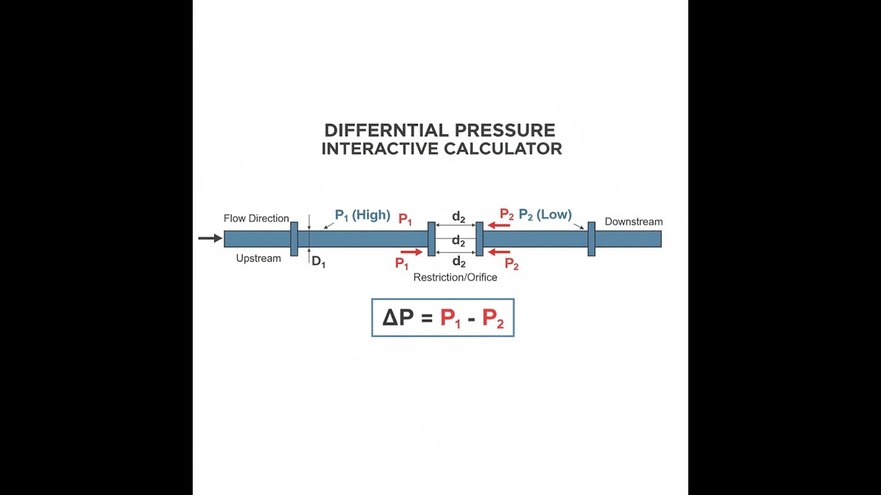
Differential pressure (ΔP) is the pressure loss as fluid moves from one point to another in a pipe or across some restriction. Usually, you measure upstream and downstream, for example before and after a filter, or across a valve. The difference tells you how much pushing force is lost getting past the obstacle.

Simple Explanation

Picture water moving through a garden hose that has a kink. Pressure will build up before the kink and drop after. That’s the differential pressure. If you make the restriction tighter or move fluid faster, the differential pressure rises. Engineers look at this value when checking flow, spotting a clogged filter, or working out what size pump they'll need.

📐 Browse all 1000+ Interactive Calculators

System Diagram

Differential Pressure Calculator

How to Use This Calculator

1. Select your calculation mode from the dropdown — choose from differential pressure, flow rate, upstream/downstream pressure, pipe pressure drop, or filter ΔP.
2. Enter the required inputs that appear for your selected mode — these may include pressures, fluid density, pipe diameter, orifice diameter, flow rate, viscosity, or filter geometry.
3. Confirm your units match those shown next to each field (kPa, m, kg/m³, etc.).
4. Click Calculate to see your result.

<> Embed this calculator → <> Embed this animation calculator →

Core Equations

Use the formula below to calculate differential pressure.

Use the formula below to calculate orifice flow rate from differential pressure.

Use the formula below to calculate pressure drop in a pipe using the Darcy-Weisbach method.

Use the formula below to calculate filter differential pressure using Darcy's Law.

Simple Example

Upstream pressure P₁ = 200 kPa. Downstream pressure P₂ = 150 kPa.
ΔP = 200 − 150 = 50 kPa (= 7.25 psi = 0.5 bar).
That 50 kPa is the differential pressure across the restriction — whether it's a valve, filter, or section of pipe.

Theory & Practical Applications

Fundamental Physics of Differential Pressure

Differential pressure is just the pressure drop between two spots in a fluid system. This idea is simple, but the details matter. In real applications, you'll see pressure loss from friction in the pipe walls, turbulence, and restrictions. At the core, you're looking at energy losses in the system, not just textbook conservation. In practice, measuring the pressure drop is often much easier than measuring actual velocity, and it gives you enough to calculate flow or spot trouble like blockages, provided you know the constraints and fluid properties.

When fluid speeds up through a narrower section, static pressure drops. But most systems aren't ideal—viscous losses and turbulent mixing add more pressure loss than Bernoulli alone would predict. This is why the Darcy-Weisbach equation and the empirically-determined friction factor get used so much. In industry, you often don't have the luxury of "clean" conditions, so you lean on differential pressure because it's practical, robust, and diagnoses more than one problem at once.

Orifice Plate Flow Measurement: Practical Considerations

Orifice plates get used in industry because they’re cheap, simple, and physically tough. No moving parts means little to go wrong. Still, there's more to it than bolting on a plate: the discharge coefficient C_d isn't constant. It changes with Reynolds number, the ratio between orifice and pipe diameter (β), and where you put your pressure taps (the tap location matters more than most people realize). Standards like ISO 5167 give you ballparks, but these numbers only hold when you operate in the turbulent flow range—usually Re > 4000. Move much below that, and your numbers start to drift.

One thing often missed is that the differential pressure you measure isn’t all recoverable. Energy turns into turbulence and heat, not just static pressure. Roughly half to most of it is “lost”—meaning your pump has to make up for it with more work (and more operating cost over time). You have a tradeoff: if you want better metering accuracy (which usually means more ΔP), you burn more energy. If you want to save energy, measurement gets less accurate. In applications where you need both, venturi meters or flow nozzles can do better, offering less permanent loss, but they cost more up front and take up more space. In short: you’ll need to be clear about your priorities at the start.

Filter Differential Pressure Monitoring

If you work with filters (HVAC units, hydraulic returns, process lines), watching the ΔP across a filter is a direct way to tell when it's getting loaded or clogged. A clean filter has low ΔP, but as it fills up, ΔP climbs. Darcy’s Law fits well here: ΔP goes up linearly with flow and is inversely proportional to permeability (which drops as a filter gets dirty).

But don’t set a fixed ΔP alarm without thinking about flow rate. If you trigger a warning at 50 kPa in all situations, you may end up replacing clean filters during high flow, or running clogged filters at low flow without noticing. The engineering workaround is to normalize ΔP by flow (ΔP/Q), which gives you a “resistance” metric—this isn’t thrown off by flow swings and only rises when loading or plugging actually happens. This method is practical for extending filter life and keeping the system operating safely without frequent unnecessary service.

Compressible Flow and Critical Pressure Ratios

For liquids, you can often ignore compressibility. But when you're dealing with gases and the pressure ratio across your restriction gets much below about 0.75, density changes start to matter, and simple formulas miss the mark. For orifice meters on gas, ISO 5167 recommends applying an expansion factor to account for this. Things change even more when the pressure ratio P₂/P₁ drops low enough (for air, roughly below 0.528)—at that stage, you reach choked (sonic) flow where mass flow maxes out, no matter how much you drop the downstream pressure.

In real equipment: If you're sizing safety valves or pneumatic controls, you need to know when you hit this choked flow limit. At that point, downstream pressure changes don't affect the flow—the upstream supply sets your maximum. This is a key check for system safety and to avoid overestimating what your pressure relief or control valve can actually pass in an upset event.

Industrial Applications Across Sectors

In pharmaceutical plants, small differential pressures separate clean rooms; gradients as small as 15–25 Pa are critical, and the difference between rooms is carefully monitored. Transmitter accuracy here needs to be tight, since getting it wrong can mean shutdowns or batch loss.

Aerospace hydraulics rely on differential pressure to see if filters are clogging and if the bypass valve needs to open—these aren’t just nice-to-have features, but essential to keep flight-critical systems working. Typical setpoints are between 200–350 kPa, and if the limit is reached, flow bypasses the filter to maintain actuation (accepting the risk of running on unfiltered fluid for a short time).

In water treatment, ΔP across filtration membranes guides when to backwash. Dirt and fouling raise ΔP over time. Once it hits about 70–80% of the rated safe limit for the membrane, the control system triggers a cleaning cycle. Adjusting backwash timing based on ΔP instead of a timer reduces wasted water and extends membrane lifetime—no advanced controls, just good use of basic instrumentation readings.

Fully Worked Engineering Example: Filter Sizing for Hydraulic System

Problem: A mobile hydraulic system requires a return line filter to protect the pump from contamination. The system operates at a maximum flow rate of 95 L/min (0.001583 m³/s) using ISO VG 46 hydraulic oil (density ρ = 875 kg/m³, dynamic viscosity μ = 0.042 Pa·s at 40°C). The selected filter media has a permeability K = 2.8 × 10⁻¹¹ m², thickness t = 0.032 m, and effective filtration area A = 0.185 m². Calculate: (a) the clean filter differential pressure, (b) the differential pressure when filter permeability degrades to 40% of original due to contamination loading, (c) the filter replacement threshold if maximum allowable ΔP is 350 kPa, and (d) the permanent pressure loss assuming 15% pressure recovery.

Solution:

Part (a) — Clean Filter Differential Pressure:

Using Darcy's Law for porous media flow:

ΔP = (μQt) / (KA)

ΔP = (0.042 Pa·s × 0.001583 m³/s × 0.032 m) / (2.8 × 10⁻¹¹ m² × 0.185 m²)

ΔP = (2.128 × 10⁻⁶) / (5.18 × 10⁻¹²)

ΔP = 410,810 Pa = 410.8 kPa

Note: This exceeds the maximum allowable 350 kPa. The filter selection is inadequate. We need to recalculate required filter area:

A_required = (μQt) / (K × ΔP_max)

A_required = (0.042 × 0.001583 × 0.032) / (2.8 × 10⁻¹¹ × 350,000)

A_required = 0.217 m²

Revised calculation with A = 0.217 m²:

ΔP_clean = (0.042 × 0.001583 × 0.032) / (2.8 × 10⁻¹¹ × 0.217) = 350 kPa (at design maximum)

For proper margin, specify filter with A = 0.26 m² to provide clean ΔP approximately 75% of maximum:

ΔP_clean = (2.128 × 10⁻⁶) / (2.8 × 10⁻¹¹ × 0.26) = 292.3 kPa

Part (b) — Differential Pressure at 40% Permeability:

When filter loads with contaminant, permeability decreases. At K = 0.40 × K_original:

K_fouled = 0.40 × 2.8 × 10⁻¹¹ = 1.12 × 10⁻¹¹ m²

ΔP_fouled = (0.042 × 0.001583 × 0.032) / (1.12 × 10⁻¹¹ × 0.26)

ΔP_fouled = 730.8 kPa

This far exceeds the 350 kPa maximum and would trigger bypass or system shutdown.

Part (c) — Filter Replacement Threshold:

The filter should be replaced when ΔP reaches 350 kPa. At this threshold, we can calculate remaining permeability:

K_threshold = (μQt) / (ΔP_max × A)

K_threshold = (2.128 × 10⁻⁶) / (350,000 × 0.26) = 2.34 × 10⁻¹¹ m²

Permeability degradation = (2.34 / 2.8) = 83.6% of original

The filter retains 83.6% permeability at replacement threshold — this provides safety margin before bypass activation.

Part (d) — Permanent Pressure Loss:

With 15% pressure recovery, permanent loss is 85% of differential pressure:

ΔP_permanent = 0.85 × 292.3 kPa = 248.5 kPa (clean filter)

Power loss = ΔP × Q = 248,500 Pa × 0.001583 m³/s = 393.5 W = 0.527 HP

This represents continuous parasitic power consumption. Over 2000 hours annual operation:

Energy waste = 393.5 W × 2000 h = 787 kWh/year

At industrial electricity rates of $0.12/kWh, this costs $94.40 annually in permanent pressure loss through the filter system.

Advanced Topics: Transient Differential Pressure in Pulsating Flows

Pumps and compressors that work in pulses (piston, plunger, reciprocating types) create rapidly changing pressure—much higher than the average. Standard pressure sensors tend to show only a moving average. To spot rapid spikes that can cause piping fatigue or noise, dampeners can be added, but they're only as good as their sizing and placement. For design or troubleshooting, use a high-frequency pressure transducer (at least 10–500 Hz depending on your equipment) to catch the peaks. This is vital for root cause analysis of vibration, wear, or noise in systems with strong pulsation.

Frequently Asked Questions

Video Walkthrough - How to Use This Calculator