Financing capital equipment or a major project means you're committing to years of payments—but most borrowers only see the monthly number, not the full cost breakdown over time. Use this loan amortization schedule calculator to calculate monthly payments, total interest paid, and the complete principal-versus-interest split every period, using your loan amount, annual interest rate, and term. It matters in manufacturing equipment purchases, commercial real estate, and engineering project finance where the difference between a good deal and a costly one comes down to understanding the full repayment structure. This page includes the amortization formula, a worked example, engineering theory, and an FAQ.
What is a Loan Amortization Schedule?
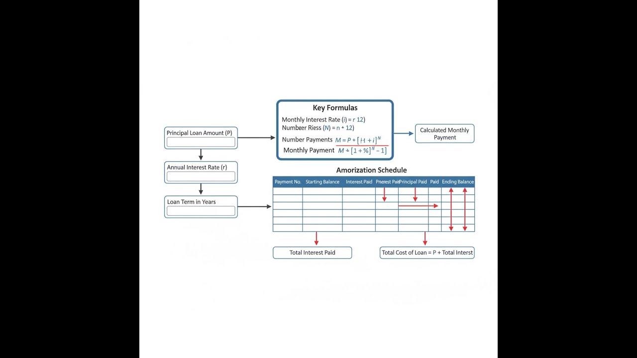
A loan amortization schedule is a table showing every payment on a loan—broken down into how much reduces your debt (principal) and how much goes to the lender as a fee for borrowing (interest). It maps the full life of the loan, payment by payment, from the first month to the last.
Simple Explanation
Think of it like eating a large meal one bite at a time. Each monthly payment is a bite—but early on, most of that bite is just the cost of sitting at the table (interest), not actually finishing the meal (paying down your debt). Over time, the balance between interest and principal flips, and more of each payment goes toward actually clearing what you owe.
📐 Browse all 1000+ Interactive Calculators
Diagram

Loan Amortization Schedule Calculator
How to Use This Calculator
- Select your Calculation Mode from the dropdown—choose from full schedule, monthly payment, loan amount, interest rate, term, or early payoff analysis.
- Enter your Loan Amount, Annual Interest Rate (%), and Loan Term (Years)—or the relevant fields for your selected mode.
- Set the Loan Start Date to align the schedule with your actual or planned start month.
- Click Calculate to see your result.
Loan Amortization Schedule Interactive Visualizer
Watch how your loan payments split between principal and interest over time. See the dramatic shift from mostly interest to mostly principal as your loan matures.
Monthly Payment
$1,688
Total Interest
$103,788
Total Cost
$303,788
FIRGELLI Automations — Interactive Engineering Calculators
Equations & Formulas
Use the formula below to calculate the fixed monthly payment for an amortized loan.
Monthly Payment Formula
M = P × [r(1 + r)n] / [(1 + r)n - 1]
Where:
M = Monthly payment ($)
P = Principal loan amount ($)
r = Monthly interest rate (annual rate ÷ 12 ÷ 100)
n = Total number of payments (years × 12)
Use the formula below to calculate the interest portion of any individual payment.
Interest Payment for Period t
It = Bt-1 × r
Where:
It = Interest payment in period t ($)
Bt-1 = Outstanding balance at beginning of period t ($)
r = Monthly interest rate
Use the formula below to calculate the principal reduction in any given payment period.
Principal Payment for Period t
PRt = M - It
Where:
PRt = Principal payment in period t ($)
M = Monthly payment ($)
It = Interest payment in period t ($)
Use the formula below to calculate the remaining loan balance after any payment.
Remaining Balance After Payment t
Bt = Bt-1 - PRt
Where:
Bt = Outstanding balance after payment t ($)
Bt-1 = Outstanding balance before payment t ($)
PRt = Principal payment in period t ($)
Use the formula below to calculate the total interest cost over the full loan term.
Total Interest Paid
Total Interest = (M × n) - P
Where:
M = Monthly payment ($)
n = Total number of payments
P = Original principal ($)
Simple Example
Loan amount: $100,000. Annual interest rate: 6%. Term: 10 years (120 payments).
Monthly rate r = 6% ÷ 12 ÷ 100 = 0.005. Monthly payment M = $1,110.21.
Month 1 interest = $100,000 × 0.005 = $500.00. Month 1 principal = $1,110.21 − $500.00 = $610.21. Remaining balance = $99,389.79.
Total paid over loan life = $133,224.60. Total interest = $33,224.60.
Theory & Engineering Applications
Loan amortization represents the systematic reduction of debt through regular, equal payments that cover both principal and interest. Unlike simple interest loans where interest is calculated only on the original principal, amortized loans use compound interest mathematics where each payment reduces the outstanding balance, which in turn reduces the interest charged in subsequent periods. This creates a dynamic payment structure where early payments consist predominantly of interest, while later payments apply increasingly larger amounts to principal reduction.
Mathematical Foundation of Amortization
The derivation of the standard amortization formula begins with the present value of an annuity equation. Each payment must satisfy the condition that the present value of all future payments equals the original loan amount. When we discount each payment M back to present value using the periodic interest rate r, we get: P = M/(1+r) + M/(1+r)² + M/(1+r)³ + ... + M/(1+r)ⁿ. This geometric series sums to P = M × [(1 - (1+r)⁻ⁿ)/r], which when solved for M yields the standard amortization payment formula.
A critical but often overlooked aspect of this formula is its sensitivity to the interest rate parameter. For a typical 30-year mortgage, a difference of just 0.5% in annual interest rate can change the total interest paid by tens of thousands of dollars. For example, on a $250,000 loan, the difference between 6.0% and 6.5% annual interest results in approximately $28,500 more in total interest paid over the life of the loan—more than 11% of the original principal. This extreme sensitivity makes accurate rate determination crucial for financial planning.
Engineering Economics and Capital Equipment Financing
In engineering project management, amortization schedules are essential for capital budgeting decisions involving equipment purchases, facility construction, and infrastructure development. The time value of money principles embedded in amortization directly impact net present value (NPV) calculations, internal rate of return (IRR) analysis, and project feasibility studies. When evaluating whether to purchase equipment outright or finance it, engineers must compare the present value of loan payments against alternative uses of capital.
For manufacturing facilities considering automation equipment, the amortization schedule reveals the true cost structure over time. A $2 million robotic assembly system financed at 7.25% over 10 years requires monthly payments of $23,476.89, with total interest of $817,227.27—representing 40.9% additional cost beyond the equipment price. However, this must be weighed against the equipment's productivity gains, labor cost savings, and the opportunity cost of deploying $2 million in working capital elsewhere. The amortization schedule helps quantify the financing burden against expected returns.
Tax Implications and Deductibility
The separation of each payment into principal and interest components has significant tax ramifications. For business loans, the interest portion is typically tax-deductible as an operating expense, while principal payments are not. This means the effective after-tax cost of borrowing is lower than the stated interest rate. For a corporation in the 21% federal tax bracket, a 6.5% interest rate effectively costs only 5.135% after accounting for the tax shield. The amortization schedule provides the precise interest amounts needed for accurate tax planning and deduction documentation.
Engineering firms financing large projects must track these schedules meticulously for financial reporting under Generally Accepted Accounting Principles (GAAP). The liability side of the balance sheet must reflect the current outstanding principal, while the income statement must accurately capture interest expense for each accounting period. Misalignment between payment dates and fiscal reporting periods requires careful accrual accounting based on the amortization schedule's period-by-period breakdown.
Worked Example: Industrial Equipment Purchase Analysis
Scenario: A precision manufacturing company needs to finance a CNC machining center costing $485,000. The equipment vendor offers financing at 7.8% annual interest over 7 years with monthly payments. The company expects the equipment to generate $9,500 per month in additional revenue and wants to understand the complete payment structure and break-even timeline.
Given Data:
- Principal amount (P) = $485,000
- Annual interest rate = 7.8%
- Loan term = 7 years = 84 months
- Expected monthly revenue = $9,500
Step 1: Calculate monthly interest rate
r = 7.8% ÷ 12 ÷ 100 = 0.0065
Step 2: Calculate monthly payment using amortization formula
M = P × [r(1 + r)ⁿ] / [(1 + r)ⁿ - 1]
M = 485,000 × [0.0065(1.0065)⁸⁴] / [(1.0065)⁸⁴ - 1]
M = 485,000 × [0.0065 × 1.7287] / [1.7287 - 1]
M = 485,000 × [0.011237] / [0.7287]
M = 485,000 × 0.015420
M = $7,478.87 per month
Step 3: Analyze first payment breakdown
Interest portion (month 1): I₁ = $485,000 × 0.0065 = $3,152.50
Principal portion (month 1): PR₁ = $7,478.87 - $3,152.50 = $4,326.37
Remaining balance: B₁ = $485,000 - $4,326.37 = $480,673.63
Step 4: Calculate total cost over loan life
Total payments = $7,478.87 × 84 = $628,225.08
Total interest paid = $628,225.08 - $485,000 = $143,225.08
Interest as percentage of principal = ($143,225.08 ÷ $485,000) × 100 = 29.5%
Step 5: Cash flow analysis
Net monthly cash flow = $9,500 - $7,478.87 = $2,021.13 positive
This positive cash flow indicates the equipment generates sufficient revenue to cover loan payments from month 1, with $2,021.13 monthly surplus for operational costs and profit.
Step 6: Analyze payment at midpoint (month 42)
First, we need the remaining balance after 41 payments. Using the remaining balance formula:
B₄₁ = P × [(1+r)ⁿ - (1+r)ᵗ] / [(1+r)ⁿ - 1]
B₄₁ = 485,000 × [(1.0065)⁸⁴ - (1.0065)⁴¹] / [(1.0065)⁸⁴ - 1]
B₄₁ = 485,000 × [1.7287 - 1.3087] / [0.7287]
B₄₁ = 485,000 × 0.5762 = $279,456.70
Interest portion (month 42): I₄₂ = $279,456.70 × 0.0065 = $1,816.47
Principal portion (month 42): PR₄₂ = $7,478.87 - $1,816.47 = $5,662.40
Notice that by the midpoint, the principal portion has increased from $4,326.37 to $5,662.40 (31% increase), while interest decreased from $3,152.50 to $1,816.47 (42% decrease). This illustrates the accelerating principal reduction characteristic of amortization.
Step 7: Engineering decision analysis
The 29.5% total interest cost must be compared against alternative financing options and the time value of money. If the company's weighted average cost of capital (WACC) is 9.5%, and the equipment has a useful life extending beyond the 7-year loan term, financing may be preferable to deploying cash reserves that could earn returns exceeding 7.8% in other investments or operational improvements. The detailed amortization schedule enables precise NPV calculations for this comparison.
This example demonstrates why engineering managers need complete amortization schedules rather than just payment amounts. The changing principal-to-interest ratio affects tax deductions, the declining balance impacts refinancing decisions, and the total interest figure is crucial for ROI calculations. For more financial engineering tools, visit our comprehensive engineering calculator library.
Early Payoff Strategies and Prepayment Impact
Extra principal payments dramatically alter amortization schedules by reducing the outstanding balance faster than scheduled, which decreases future interest charges since interest is calculated on the remaining balance. A non-intuitive consequence is that early extra payments have exponentially greater impact than later ones. An extra $200 payment in month 12 of a 30-year mortgage saves far more total interest than the same $200 extra payment in month 300, because the earlier payment reduces the balance upon which 348 subsequent interest calculations compound.
For the previous example with monthly payment of $7,478.87, adding just $500 extra principal each month reduces the loan term from 84 months to approximately 71 months (13 months early) and saves roughly $18,200 in total interest. This represents a guaranteed 7.8% return on those extra payments—equivalent to the loan's interest rate—making prepayment one of the most risk-free "investments" available when loan rates exceed conservative investment returns.
Practical Applications
Scenario: Manufacturing Facility Expansion Decision
James, a facilities manager at an automotive parts manufacturer, needs to expand production capacity by adding a $1.2 million automated paint line. The bank offers 8.5% financing over 10 years. Before committing, James uses the amortization calculator to discover the monthly payment would be $14,863.58, with total interest of $583,629.81—nearly half the equipment cost. By examining the complete payment schedule, he realizes that in year one alone, $96,847 goes to interest versus only $81,515 to principal. This detailed breakdown helps James present the true 10-year cost of $1,783,630 to the CFO, who decides to negotiate a larger down payment to reduce the financed amount to $900,000, lowering the monthly burden to $11,147.69 and saving over $146,000 in interest. The amortization schedule becomes a central document in their capital budgeting presentation to the board.
Scenario: Engineering Firm Office Building Purchase
Maria, the CFO of a 45-person civil engineering firm, is evaluating whether to purchase their office building for $875,000 rather than continuing to lease at $8,200 monthly. A commercial mortgage broker quotes 6.75% over 25 years. Using the loan amortization calculator, Maria determines the monthly payment would be $6,233.82—$1,966 less than current rent. However, the detailed amortization schedule reveals crucial insights: in the first year, $58,239 of payments go to interest while only $16,566 reduces principal. For tax planning, Maria's accountant needs these exact figures since only the interest is deductible. The calculator also shows that after 5 years, the remaining balance would still be $810,447—essential information for the firm's balance sheet projections. By running a second calculation with an extra $1,000 monthly payment, Maria discovers this would retire the loan in 18.3 years instead of 25, saving $164,832 in interest. These detailed scenarios enable the partners to make an informed decision based on complete financial understanding rather than just comparing monthly payment to rent.
Scenario: Research Equipment Financing for University Lab
Dr. Chen, a mechanical engineering professor, secured a $650,000 grant to establish a new materials testing laboratory. While the grant covers equipment purchase, the university's procurement office suggests financing the equipment at 5.25% over 5 years to preserve grant funds for operational expenses and student stipends. Dr. Chen uses the amortization calculator to analyze this option, finding monthly payments would be $12,301.74 with total interest of $88,104.55. By generating the complete payment schedule, she can align payment timing with the university's fiscal year budget cycles. The month-by-month breakdown shows that $2,843.75 of the first payment is interest—this matters because grant funds can cover interest on equipment supporting research activities. Dr. Chen presents the amortization schedule to the grants office, demonstrating that over the 5-year loan period, the lab will pay $88,104 in deductible interest while preserving $650,000 in grant principal for consumables, student support, and facility modifications that aren't financeable. The detailed schedule enables precise multi-year budget forecasting required for continued grant compliance and renewal applications.
Frequently Asked Questions
▼ Why does most of my payment go to interest in the early years?
▼ How much can I really save by making extra principal payments?
▼ Should I use extra cash to pay down my loan or invest it elsewhere?
▼ What's the difference between amortization and simple interest loans?
▼ How do I use an amortization schedule for tax reporting?
▼ Can I calculate the interest rate if I only know the payment amount?
Free Engineering Calculators
Explore our complete library of free engineering and physics calculators.
Browse All Calculators →🔗 Explore More Free Engineering Calculators
About the Author
Robbie Dickson — Chief Engineer & Founder, FIRGELLI Automations
Robbie Dickson brings over two decades of engineering expertise to FIRGELLI Automations. With a distinguished career at Rolls-Royce, BMW, and Ford, he has deep expertise in mechanical systems, actuator technology, and precision engineering.
Need to implement these calculations?
Explore the precision-engineered motion control solutions used by top engineers.


