Diopter Interactive Calculator

The diopter calculator determines optical power, focal length, and image formation characteristics for lenses and optical systems. Optometrists, ophthalmologists, optical engineers, and photographers use diopter calculations daily to specify corrective lenses, design imaging systems, and predict image location. This calculator handles lens power conversion, focal length determination, object-image conjugate relationships, and lens combination effects across multiple calculation modes.

📐 Browse all free engineering calculators

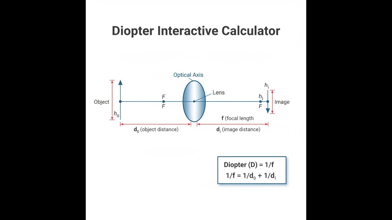
Optical System Diagram

Diopter Calculator

Governing Equations

Theory & Practical Applications

The diopter represents a fundamental unit in optics that elegantly unifies the concepts of optical power, focal length, and wavefront curvature into a single reciprocal-length quantity. Unlike focal length, which requires conversion between millimeters and meters depending on application context, diopter values remain consistent and directly additive when thin lenses are placed in contact — a property that makes prescription calculations and optical system design dramatically simpler. The definition P = 1/f (where f is in meters) establishes a clear inverse relationship: strong lenses with short focal lengths have high diopter values, while weak lenses with long focal lengths have low diopter values. This reciprocal formulation means that a +2.0 D lens has twice the optical power of a +1.0 D lens, providing intuitive scaling for optical professionals.

Sign Conventions and Physical Interpretation

The sign of diopter power encodes critical information about lens behavior. Positive diopters (+D) indicate converging lenses with real focal points — these lenses bend parallel incident rays toward a point on the opposite side. The +2.5 D reading glasses commonly prescribed for presbyopia have a focal length of 0.40 meters (40 cm), meaning parallel rays converge at this distance. Negative diopters (−D) represent diverging lenses that spread parallel rays as if they originated from a virtual focal point on the incident side. A −3.0 D myopia correction lens has a focal length of −0.333 meters, creating virtual images of distant objects at comfortable viewing distances. This sign convention extends to vergence calculations: light converging toward a point has positive vergence, while diverging light has negative vergence. Understanding that object distance vergence equals −1/d_o (negative because light approaches the lens) while image vergence equals +1/d_i (positive for real images) prevents systematic sign errors that plague novice optical designers.

The Thin Lens Equation and Conjugate Relationships

The thin lens equation 1/f = 1/d_o + 1/d_i expresses the fundamental conjugate relationship between object and image positions. When manipulated into vergence form (P = U_out − U_in), this equation reveals that lens power equals the change in wavefront vergence produced by the refractive surface. For a +5.0 D lens with an object at 0.25 m, the input vergence U_in = −1/0.25 = −4.0 D (negative approaching), output vergence U_out = −4.0 + 5.0 = +1.0 D, yielding an image distance d_i = 1/1.0 = 1.0 m. This vergence approach proves particularly valuable in complex systems where tracking individual ray paths becomes cumbersome. A critical but often overlooked limitation emerges at the focal distance: when d_o = f, the denominator (d_o − f) approaches zero, image distance trends toward infinity, and the lens produces collimated output — this condition defines the boundary between real and virtual image formation.

Compound Lens Systems and Effective Power

When two thin lenses separated by distance d combine, their effective power follows P_eff = P₁ + P₂ − d·P₁·P₂, deviating from simple addition due to the finite separation term. Consider a +6.0 D objective and +20.0 D eyepiece separated by 0.025 m (25 mm) in a microscope: contact power would yield P_contact = +26.0 D, but actual effective power P_eff = 6.0 + 20.0 − (0.025)(6.0)(20.0) = 23.0 D — a 3.0 D reduction representing the geometric spacing effect. This separation term dominates in telephoto lens designs where negative and positive elements interact: a +10.0 D front element paired with a −5.0 D rear element at 0.08 m separation yields P_eff = 10.0 + (−5.0) − (0.08)(10.0)(−5.0) = 5.0 + 4.0 = +9.0 D, with the positive separation term actually increasing power. Optical engineers exploit this effect to achieve compact form factors with long effective focal lengths — critical for telephoto camera lenses and laser beam expanders where physical length constraints preclude single-element solutions.

Magnification and Image Properties

Linear magnification m = −d_i/d_o quantifies image size relative to object size, with the negative sign encoding orientation inversion. Real images (positive d_i) always exhibit negative magnification, appearing inverted, while virtual images (negative d_i) show positive magnification and remain upright. For machine vision applications requiring precise dimensional measurements, this magnification must be calibrated against known reference standards since focal length tolerances typically range ±1–2% in commercial optics. A +50.0 D (20 mm focal length) lens imaging an object at 30 mm produces image distance d_i = f·d_o/(d_o − f) = (0.020)(0.030)/(0.030 − 0.020) = 0.060 m = 60 mm, yielding magnification m = −60/30 = −2.0×. The image appears twice as large and inverted. Angular magnification M_θ differs from linear magnification and proves more relevant for visual instruments — a 10× microscope objective doesn't produce 10× linear magnification at the image plane but rather provides 10× angular magnification when viewed through the eyepiece, accounting for the entire optical system including the observer's eye.

Ophthalmic Applications and Prescription Optimization

Eyeglass prescription optimization requires accounting for vertex distance — the separation between the back surface of the corrective lens and the eye's cornea. Standard refraction measurements occur at approximately 12–14 mm vertex distance, but frame selection alters this distance, changing effective power at the corneal plane. For high prescriptions exceeding ±4.0 D, vertex distance compensation becomes critical: a −8.0 D lens placed 14 mm from the eye delivers effective power P_eff = P/(1 − d·P) = −8.0/(1 − 0.014·(−8.0)) = −8.0/1.112 = −7.19 D at the cornea — a 0.81 D error that significantly impacts visual acuity. Contact lenses eliminate this issue by positioning the corrective power directly at the cornea, but introduce their own considerations: soft contact lenses flex on the eye, effectively adding ±0.25 to ±0.50 D of astigmatic power depending on material stiffness and eye geometry. Optometrists routinely perform vertex corrections when converting between spectacle and contact lens prescriptions, particularly for aphakic patients requiring +10.0 to +14.0 D corrections post-cataract surgery.

Industrial Imaging and Machine Vision

Industrial machine vision systems employ diopter calculations for working distance optimization and depth of field management. A typical quality control station imaging 50 mm components might use a +100.0 D (10 mm focal length) lens at 15 mm working distance. The thin lens equation yields d_i = (0.010·0.015)/(0.015 − 0.010) = 0.030 m = 30 mm behind the lens, producing m = −30/15 = −2.0× magnification on a 1/2" sensor (6.4 mm × 4.8 mm imaging area). This setup covers 3.2 mm × 2.4 mm object space — adequate for many defect detection tasks. Depth of field DoF ≈ 2·N·c·(d_o/f)² constrains focus tolerance, where N represents f-number (f/D with D as aperture diameter) and c denotes circle of confusion criterion. For N=8, c=0.01 mm, f=10 mm, d_o=15 mm: DoF ≈ 2·8·0.01·(15/10)² = 0.36 mm — extremely shallow, demanding precision positioning systems. Telecentric lenses modify this equation by placing the aperture stop at the focal plane, producing orthographic projection where magnification remains constant across depth variations, essential for accurate dimensional metrology.

Laser Beam Shaping and Collimation

Laser systems utilize diopter calculations for beam collimation and focusing. A typical laser diode emits a diverging beam characterized by fast and slow axis divergence angles — often 25° × 10° FWHM (full width half maximum). Collimating this beam requires positioning the diode at the focal point of a collimating lens. For a +100.0 D (10 mm) collimator, the diode must sit precisely 10.00 mm from the lens principal plane, within ±0.05 mm tolerance to maintain <5 mrad residual divergence. Focusing high-power industrial cutting lasers involves inverse calculations: to achieve a 0.1 mm diameter focal spot from a 10 mm collimated beam requires focal ratio f/D = 1/(2·θ·D) where θ represents focused spot size in radians. For D=10 mm beam and 0.1 mm spot: required focal length f = 0.1·10/(10·tan(θ)) ≈ 10 mm, corresponding to +100.0 D focusing optic. Thermal lensing in high-power systems — where absorbed energy changes refractive index — can shift effective focal length by several diopters, requiring active focus compensation via adjustable optics or thermally-optimized lens designs.

Fully Worked Example: Compound Microscope Optical Design

Design a compound microscope using commercially available lenses to achieve 40× total magnification with 160 mm tube length (standard optical distance from objective rear focal point to eyepiece front focal point). Objective specifications: +25.0 D (+0.04 m = 40 mm focal length), specimen at 42 mm working distance. Eyepiece specifications: +50.0 D (20 mm focal length) for comfortable viewing.

Step 1: Calculate objective image distance
Using thin lens equation with d_o = 0.042 m, f_obj = 0.040 m:
1/d_i = 1/f − 1/d_o = 1/0.040 − 1/0.042 = 25.0 − 23.81 = 1.19 m⁻¹
d_i = 0.840 m = 840 mm

Problem: This violates the 160 mm tube length requirement. Recalculate with corrected working distance.

Step 2: Determine required object distance for 160 mm image distance
Target d_i = 0.160 m, f_obj = 0.040 m:
1/d_o = 1/f − 1/d_i = 25.0 − 6.25 = 18.75 m⁻¹
d_o = 0.0533 m = 53.3 mm working distance

Step 3: Calculate objective magnification
m_obj = −d_i/d_o = −160/53.3 = −3.00×

Step 4: Determine eyepiece magnification
For 40× total magnification: M_total = |m_obj| · M_eyepiece
M_eyepiece = 40/3.00 = 13.3×

Step 5: Verify eyepiece design
Standard eyepiece angular magnification M_ep = 250 mm / f_ep where 250 mm represents near point distance:
M_ep = 250/20 = 12.5× (close to required 13.3×)

Step 6: Calculate effective system parameters
Total optical length = working distance + tube length + eyepiece focal length
L_total = 53.3 + 160 + 20 = 233.3 mm

Step 7: Determine field of view
For 10 mm eyepiece field stop diameter:
Object space field = field stop / |m_obj| = 10/3.00 = 3.33 mm diameter

Engineering Insight: The actual achieved magnification of 37.5× (using standard 12.5× eyepiece) differs from the target 40×, demonstrating why microscope manufacturers offer multiple objective/eyepiece combinations rather than expecting arbitrary values to match exactly. Professional microscopy laboratories stock objectives in standardized magnifications (4×, 10×, 20×, 40×, 100×) and eyepieces (8×, 10×, 12.5×, 16×) to achieve predictable system performance. Infinity-corrected modern microscopes place the objective image at infinity (collimated space) between objective and eyepiece, allowing insertion of filters, polarizers, and beam splitters without affecting focus — a critical advantage for advanced imaging modalities like fluorescence and differential interference contrast.

Additional resources on optical calculations are available in the engineering calculator library, including lens design optimization tools and aberration analysis utilities.

Frequently Asked Questions