Optical Density Interactive Calculator

The Optical Density Interactive Calculator enables precise determination of light transmission, absorption, and refractive properties through optical media. Essential for spectroscopy, photometry, filter design, and optical system engineering, this tool calculates optical density (OD), transmittance, absorbance, and related parameters across multiple calculation modes. Engineers in telecommunications, laboratory instrumentation, photography, and laser systems rely on optical density calculations for accurate light attenuation specifications and quality control.

📐 Browse all free engineering calculators

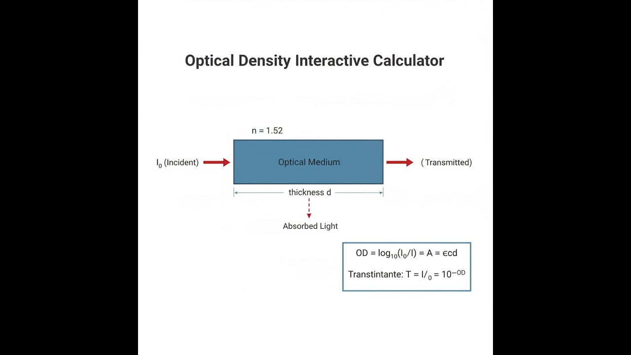
Optical Density Diagram

Interactive Optical Density Calculator

Equations & Variables

Theory & Practical Applications

Fundamental Physics of Optical Density

Optical density quantifies the attenuation of electromagnetic radiation as it propagates through an absorbing medium. Unlike simple geometric opacity, optical density accounts for the logarithmic relationship between incident and transmitted light intensity, reflecting the exponential decay of photon flux described by the Beer-Lambert law. When light encounters matter, photons interact with electrons in atoms and molecules through absorption, scattering, and re-emission processes. The probability of photon absorption over a differential path length is proportional to the number density of absorbing species and their absorption cross-section at the incident wavelength.

The logarithmic definition OD = log₁₀(I₀/I) ensures that optical densities are additive for series-arranged optical elements—a critical property for filter stacking and multi-stage optical systems. A filter with OD 2.0 reduces intensity by a factor of 100 (transmittance T = 0.01), while two such filters in series produce OD 4.0 with T = 0.0001. This multiplicative transmittance behavior (T_total = T₁ × T₂) transforms into additive optical density (OD_total = OD₁ + OD₂), simplifying system design calculations. Engineers working with laser safety eyewear must account for this additive property when specifying protection levels against specific wavelengths.

The Beer-Lambert law A = εcd establishes the linear relationship between absorbance and concentration, making spectrophotometry a quantitative analytical technique. The molar absorptivity ε characterizes how strongly a chemical species absorbs light at a given wavelength and is an intrinsic molecular property determined by electronic transition probabilities. For biomolecules, ε values at characteristic wavelengths enable protein concentration determination: bovine serum albumin exhibits ε_280nm ≈ 43,824 L·mol^-1·cm^-1, allowing nanogram-level detection in 1 cm cuvettes. Deviations from Beer-Lambert linearity occur at high concentrations due to molecular interactions, refractive index changes, and polychromatic illumination effects.

Spectroscopic Applications and Instrumentation

UV-visible spectrophotometry exploits optical density measurements across 200-800 nm wavelengths to identify and quantify chemical compounds. DNA concentration analysis relies on the strong absorption peak at 260 nm (ε ≈ 6600 L·mol^-1·cm^-1 per nucleotide), with the A₂₆₀/A₂₈₀ ratio indicating sample purity—pure DNA yields ratios of 1.8, while protein contamination reduces this value. Microvolume spectrophotometers using 0.5-2 μL samples and 0.05-1.0 mm path lengths have revolutionized molecular biology workflows, enabling concentration measurements from 2-15,000 ng/μL without dilution. The short path length accommodates the modified Beer-Lambert relationship where high concentrations remain within the linear detection range (OD typically 0.1-1.5 for optimal accuracy).

In optical filter manufacturing, neutral density (ND) filters are specified by their optical density or equivalent filter factor. An ND 1.0 filter reduces intensity by one order of magnitude (T = 0.1, filter factor 10×), while ND 3.0 achieves 1000× attenuation. Variable ND filters constructed from rotating polarizers provide continuously adjustable attenuation through Malus's Law (T = cos²θ), though this introduces polarization-dependent effects. Metallic and absorptive glass ND filters maintain spectral neutrality across visible wavelengths but exhibit wavelength-dependent absorption in UV and IR regions, requiring calibration curves for broadband applications. Solar observation telescopes commonly employ ND 5.0 filters (100,000× attenuation) to prevent retinal damage and detector saturation.

Telecommunications and Optical Power Budgets

Fiber optic communication systems express optical power loss in decibels (dB), which relates to optical density through the conversion factor 1 OD = 10 dB. A 10 km fiber span with 0.2 dB/km attenuation produces 2 dB total loss (OD = 0.2, T = 0.631), reducing signal power by 36.9%. Link budget calculations account for splice losses (0.05-0.1 dB), connector losses (0.3-0.5 dB), and component insertion losses alongside fiber attenuation. Single-mode fibers operating at 1550 nm achieve minimum attenuation of 0.17 dB/km due to reduced Rayleigh scattering, enabling spans exceeding 80 km without amplification. Dispersion-compensating fibers with higher doping concentrations exhibit elevated attenuation (0.4-0.5 dB/km), requiring optimization between chromatic dispersion compensation and optical power budget.

Erbium-doped fiber amplifiers (EDFAs) provide 20-40 dB gain in C-band (1530-1565 nm) telecommunications windows, compensating for accumulated transmission losses in long-haul networks. Optical add-drop multiplexers introduce 3-6 dB insertion loss per channel, constraining network architectures to specific reach limitations. Dense wavelength-division multiplexing (DWDM) systems with 40-96 channels require precise optical power equalization across wavelengths—variations exceeding 1 dB degrade bit error rates and reduce system margin. Automated gain control maintains per-channel power within ±0.5 dB through dynamic attenuation and amplifier pump current adjustment.

Laser Safety and Ocular Hazard Assessment

Laser safety eyewear selection depends on optical density at the laser wavelength sufficient to reduce irradiance below the maximum permissible exposure (MPE) level. For a Class 4 laser emitting 5 W at 532 nm (continuous wave) with 3 mm beam diameter, the irradiance is 70.7 kW/cm². The MPE for 532 nm continuous exposure is 2.5 mW/cm², requiring attenuation by a factor of 28,280, corresponding to OD = 4.45. Safety regulations mandate minimum OD 5.0 eyewear with additional 0.5 OD safety margin, ensuring worst-case scenarios including beam reflections remain below MPE. Pulsed lasers require higher OD specifications due to peak power considerations—a 10 ns Q-switched Nd:YAG laser (1064 nm) with 100 mJ pulse energy may demand OD 7-9 eyewear depending on repetition rate and exposure geometry.

Wavelength-dependent absorption mechanisms in laser safety filters rely on absorptive dyes, dielectric multilayer coatings, or holographic gratings. Absorptive filters exhibit broad rejection bands but risk thermal damage under high-power exposure, while dielectric coatings provide sharper cutoff characteristics and higher damage thresholds exceeding 10 J/cm². The visible light transmission (VLT) specification balances safety requirements against operational visibility—OD 6+ filters at specific laser wavelengths may transmit 10-40% of ambient light in non-hazardous spectral regions, maintaining adequate workspace illumination. Calibration drift and UV-induced degradation necessitates annual spectrophotometric verification of rated OD performance.

Photography and Cinematography

Neutral density filters enable long-exposure photography in bright conditions and shallow depth-of-field cinematography at wide apertures. A 6-stop ND filter (ND 1.8, T = 0.0158) allows f/1.4 aperture shooting in bright sunlight while maintaining 1/50 s shutter speed for natural motion blur in 24 fps video. Variable ND filters constructed from crossed linear polarizers provide 2-8 stop range but introduce cross-polarization artifacts at extreme attenuation settings—the "X pattern" vignetting visible in wide-angle lenses results from ray angle-dependent polarization states interacting with the crossed filter elements. Fixed ND filters fabricated from absorptive glass or metallic coatings avoid polarization effects but lack adjustment flexibility.

Graduated ND filters with spatial density variation balance exposure between bright skies and darker foregrounds in landscape photography. A 3-stop hard-edge graduated ND (transition zone 1-2 mm) compresses 8 EV scene dynamic range to 5 EV sensor capability, preventing highlight clipping while maintaining shadow detail. Soft-edge graduated filters (10-15 mm transition) suit irregular horizons but require precise filter positioning to avoid visible density boundaries. Digital blending techniques using multiple exposures have reduced graduated ND usage, though physical filters remain preferred for maintaining authentic in-camera image quality and avoiding motion artifacts in scenes with moving elements.

Worked Example: Spectrophotometric Protein Quantification

Problem: A biochemistry laboratory receives an unknown protein sample and must determine its concentration using UV spectrophotometry. The protein has a known molar absorptivity ε_280nm = 35,200 L·mol^-1·cm^-1 and molecular weight MW = 45,000 g/mol. A technician dilutes the sample 1:10 in phosphate buffer and measures the absorbance in a standard 1.0 cm quartz cuvette. The spectrophotometer reading shows A₂₈₀ = 0.847. Calculate: (a) the molar concentration of the diluted sample, (b) the mass concentration in mg/mL of the diluted sample, (c) the original stock concentration in mg/mL, and (d) the transmittance and percent light absorbed at 280 nm.

Solution:

(a) Molar concentration of diluted sample:
Using the Beer-Lambert law A = εcd, we solve for concentration:
c = A / (εd)
c = 0.847 / (35,200 L·mol^-1·cm^-1 × 1.0 cm)
c = 0.847 / 35,200 L·mol^-1
c = 2.406 × 10^-5 mol/L = 24.06 μM

(b) Mass concentration of diluted sample:
Convert molar concentration to mass concentration using molecular weight:
Mass concentration = c × MW
Mass concentration = (2.406 × 10^-5 mol/L) × (45,000 g/mol)
Mass concentration = 1.083 g/L = 1.083 mg/mL

(c) Original stock concentration:
Account for the 1:10 dilution factor:
Stock concentration = Diluted concentration × Dilution factor
Stock concentration = 1.083 mg/mL × 10
Stock concentration = 10.83 mg/mL

(d) Transmittance and percent absorbed:
Transmittance: T = 10^-A = 10^-0.847 = 0.1422 = 14.22%
Percent absorbed = (1 - T) × 100% = (1 - 0.1422) × 100% = 85.78%

Verification and practical considerations: The measured absorbance of 0.847 falls within the optimal linear range (0.1-1.5 OD) for most spectrophotometers, ensuring measurement accuracy within ±2%. If the absorbance exceeded 1.5, further dilution would be required to maintain linearity. The 1:10 dilution strategy proves appropriate, as direct measurement of the stock solution would yield A = 8.47, far exceeding detector linearity limits. For increased accuracy, triplicate measurements with averaged results and blank correction (buffer-only measurement subtracted) are standard practice. Temperature control at 25°C ± 0.5°C prevents thermochromic shifts in absorption spectra that could introduce systematic errors of 1-3% in ε values.

This example demonstrates typical protein quantification workflow in molecular biology and pharmaceutical development. For samples with unknown molar absorptivity, Bradford or bicinchoninic acid (BCA) colorimetric assays provide concentration estimates using standard curves constructed from known protein standards like bovine serum albumin.

Frequently Asked Questions