If you don’t have good cycle time numbers when designing a robotic work cell, you’re setting yourself up for missed production targets—and you might not find out until the line is already built. This Robot Cycle Time & Throughput Estimator lets you quickly estimate total cycle time and the parts-per-hour output using the main time segments—load, unload, process, each robot motion, and a practical safety factor. The difference between calculated and actual cycle times, even at just 10%, can cause real headaches in places like automotive assembly or electronics manufacturing, where every second counts. Below, you'll find the math, an example, details for engineers, and an FAQ.
What is robot cycle time?
Robot cycle time is how long the robot actually takes to go from starting one part to starting the next, including every move and operation. This is the number that sets your maximum possible throughput.
Simple Explanation
Imagine following a recipe step by step: pick the part up, move it, process it, return the arm, and reset. Add up the time for every action, tack on some extra for inevitable small delays, and you’ve got the cycle time. Shorter cycles mean higher output.
📐 Browse all 384 free engineering calculators
Robot Motion Sequence Diagram

Robot Cycle Time Calculator
How to Use This Calculator
This calculator is intended for education, concept evaluation, and preliminary design. Results are based on the equations and assumptions described on this page, but cannot account for every real-world load case, tolerance, material property, environmental condition, installation detail, safety factor, code, or regulatory requirement. Verify all inputs, assumptions, units, and results independently before selecting components or using the result in a real application. Safety-critical, structural, medical, lifting, transportation, or regulated applications must be reviewed by a qualified engineer.
- Enter the load time, unload time, and process time in seconds.
- Enter all robot motion segment times as comma-separated values (e.g., 3.2, 1.8, 2.5).
- Set your safety factor — use 1.1 for simple systems, up to 1.3 for complex multi-sensor setups.
- Click Calculate to see your result.
Input Parameters
📹 Video Walkthrough — How to Use This Calculator
Robot Cycle Time Interactive Visualizer
Visualize how motion times, process times, and safety factors combine to determine total robot cycle time and production throughput. Adjust parameters to see real-time impact on parts-per-hour output.
CYCLE TIME
23.0 s
PARTS/HOUR
157
DAILY OUTPUT
2,512
FIRGELLI Automations — Interactive Engineering Calculators
Mathematical Equations
Here are the basic relationships for cycle time and throughput.
Core Cycle Time Equations
Tmotion = Σ tmove,i
Sum of all individual motion segment times
Tprocess = tload + toperation + tunload
Sum of material handling and processing operations
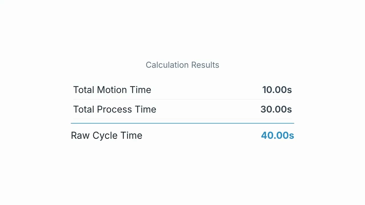
Traw = Tmotion + Tprocess
Basic theoretical cycle time
Tcycle = Traw × SF
Where SF is the safety factor (typically 1.1-1.2)
PPH = 3600 / Tcycle
Parts per hour based on cycle time in seconds
Simple Example
Given: Load time = 2 s, Unload time = 2 s, Process time = 10 s, Motion times = 3 s + 3 s = 6 s, Safety factor = 1.1
- Total process time: 2 + 2 + 10 = 14 s
- Total motion time: 6 s
- Raw cycle time: 14 + 6 = 20 s
- Adjusted cycle time: 20 × 1.1 = 22 s
- Parts per hour: 3600 ÷ 22 = 164 parts/hr
Technical Analysis and Applications
Understanding Robot Cycle Time Optimization
The only way to properly size and justify a robotic system is to map out all the cycle steps, time them, and calculate what can realistically be achieved. Using this calculator, you can add up your motion paths, process steps, and handling times to get a throughput estimate that actually reflects what happens on the floor—not just in the brochure. This matters most at the quoting and debottlenecking stage, and is crucial if you actually need to hit daily or hourly targets.
Motion Time Components and Analysis
Each move the robot makes typically has three parts: acceleration (off the line from stop), steady motion at the set max speed, and then deceleration into a stop. Industrial robots use acceleration profiles—like trapezoidal or smoothed S-curves—so you don’t stress the joints or create unnecessary vibration. For most shop-floor arms, you’ll see 1–3 m/s for linear travel and 180–360°/s for turning, but payload and needed accuracy will knock that down. When programming, the controller picks all this up and can tweak for obstacles, path constraints, or even jerk limits if you demand gentle handling. For any moves done with FIRGELLI linear actuators, the focus shifts to precise end-position and stable, consistent control since these often set throughput on fine-adjustment or clamping steps.
Process Time Optimization Strategies
Process time is all the time that isn’t robot movement—gripping, clamping, welding, inspection, or waiting for another machine. These times are often dictated by other equipment you interface with, not the robot itself. Tuning these steps is usually more about smarter sequencing in the controller, parallel operations with good mechanical design, or fast feedback via industrial networks. You can often get a little more speed with better end effector (gripper) designs, more reliable part presentation, and combining vision with robot moves so positioning isn’t as tentative. Don’t undersize grippers or actuators to chase speed; consistently reliable operation is usually more valuable.
Safety Factor Considerations
The safety factor covers all the real-world slowdowns that catch up with you—temperature drift, mechanical wear, changing payload, network lag, retries, and moments when things just don’t move as fast as you modeled. You might get away with 1.1 on a basic point-to-point pick-and-place, but more sensors, more tools, or processes running in tandem make you want to push that up to 1.2 or higher. If things are fiddly or sequence timing keeps changing, budgeting extra will save you arguments later. Don’t take out all the slack: leave enough room so the system outperforms what’s on paper, not the other way around.
Practical Application Example
Take an automotive robot that installs door panels. It moves from home to the parts conveyor (2.1 seconds), picks up the panel (1.8 seconds for approach and grip), swings it to the vehicle (3.4 seconds), aligns with vision (2.2 seconds), installs (4.5 seconds), then returns and resets (2.8 seconds).
Calculate it out:
- Motion times: 2.1 + 3.4 + 2.8 = 8.3 seconds
- Process times: 1.8 + 2.2 + 4.5 = 8.5 seconds
- Raw cycle time: 8.3 + 8.5 = 16.8 seconds
- Adjusted cycle time: 16.8 × 1.15 = 19.3 seconds
- Production rate: 3600 ÷ 19.3 = 187 parts per hour
If your analysis shows motion and process times are close, the system is pretty balanced. If motion dominates, look at faster paths or higher acceleration; if process time dominates, consider if steps can be decoupled, sequenced in parallel, or sped up by tooling changes.
Advanced Optimization Techniques
Running more than one robot in parallel, especially if you set it up so one’s moving while the other is processing or prepping parts, will increase throughput—but only if the control system is up to managing them. Don’t forget that adding robots means adding coordination overhead, and that requires more advanced programming and sometimes network upgrades. On the maintenance side, tracking trends—like rising motion times—through vibration or thermal sensors is the only way to catch creeping wear before it catches you. Paths can also be re-optimized: you can get real gains by refining robot motion profiles and avoiding joint limits or unnecessary clearance; sometimes this shaves 5–15% off cycle time after installation, not just at commissioning.
Integration with Manufacturing Systems
Cycle time isn’t just the robot—it’s the entire cell. Conveyor speed, feeder timing, and what’s happening downstream can be rate-limiting. Mapping every stage and doing a bottleneck analysis helps you avoid blaming the robot for problems that actually originate somewhere else. With modern controls, you can pull cycle data off the line in real time and start to spot patterns or drift, using that to fine-tune or flag upcoming issues before they cost production hours.
Economic Impact and ROI Considerations
Cycle time feeds directly into ROI. A 10% cycle time error will be noticed on an annual production schedule and can translate to thousands of parts lost or late. If you improve cycle time—by whatever percent—you either get more product out or do the same work with less wear and less energy. Fast acceleration profiles will bump up peak energy draw but can actually lower total energy per part by running more efficiently overall. Drives with regeneration can re-capture energy during braking, but this only pays off if you’re running enough cycles to matter.
Frequently Asked Questions
📐 Explore our full library of 384 free engineering calculators →
About the Author
Robbie Dickson
Chief Engineer & Founder, FIRGELLI Automations
Robbie Dickson brings over two decades of engineering expertise to FIRGELLI Automations. With a distinguished career at Rolls-Royce, BMW, and Ford, he has deep expertise in mechanical systems, actuator technology, and precision engineering.
🔗 Explore More Free Engineering Calculators
Need to implement these calculations?
Explore the precision-engineered motion control solutions used by top engineers.


