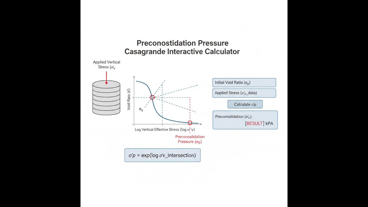
Preconsolidation Pressure Casagrande Interactive Calculator

Results

Why does the Casagrande method require plotting void ratio versus LOG of stress rather than arithmetic stress? +

The logarithmic stress axis reveals the fundamental compression behavior that would be obscured on an arithmetic plot. Soil compression follows a roughly logarithmic relationship with stress because the mechanism involves progressive collapse of larger void spaces first, followed by smaller voids at higher stresses — a geometric progression. On a log scale, the virgin compression line appears nearly straight over typical engineering stress ranges, making identification of the preconsolidation point much clearer as a distinct break in slope. On an arithmetic plot, the curve would show continuous curvature with no obvious transition point, making systematic identification of preconsolidation pressure impossible. Additionally, the logarithmic representation compresses the high-stress region and expands the low-stress region where the critical recompression-to-virgin-compression transition occurs, providing better resolution exactly where engineers need it most. The semi-log plot also reflects the exponential nature of particle rearrangement processes and aligns with theoretical models of soil compressibility derived from statistical mechanics of granular materials.

How accurate is the Casagrande method, and what factors affect the reliability of preconsolidation pressure determination? +

The Casagrande method typically provides preconsolidation pressure estimates within 15 to 25 percent of the "true" value when applied to high-quality undisturbed samples of moderately to heavily overconsolidated clays. However, this accuracy degrades substantially for lightly overconsolidated soils (OCR less than 2) where the transition from recompression to virgin compression is very gradual, making identification of the maximum curvature point highly subjective. Sample disturbance represents the most critical limitation — tube sampling inevitably causes some stress relief and structure disruption, which softens the material and can shift the apparent preconsolidation pressure downward by 20 to 40 percent in sensitive clays. Block sampling or in-situ testing methods provide better data but are expensive. The operator's skill in constructing the tangent, horizontal, and bisector lines introduces additional variability; studies show that different experienced engineers analyzing the same consolidation curve may report preconsolidation pressures varying by 10 to 20 percent. For these reasons, geotechnical practice typically involves testing multiple samples from a layer and using engineering judgment to select representative values, rather than relying on a single test result. The method works best for stiff overconsolidated clays with sharp transitions and becomes increasingly uncertain for soft, lightly overconsolidated, or highly disturbed samples.

What does it mean when calculated OCR is less than 1.0, and how should engineers respond? +

An OCR less than 1.0 is physically impossible because it would imply the soil is currently stressed beyond any stress it has previously experienced — contradicting the definition of preconsolidation pressure as the maximum past stress. When calculations yield OCR less than 1.0, it indicates a problem with either the data or the analysis. Common causes include: incorrectly calculated in-situ effective stress (often from wrong water table elevation or unit weight), misidentification of the preconsolidation point on the consolidation curve (selecting a point too far left, giving artificially low σ'_p), severe sample disturbance that destroyed the overconsolidated structure, or transcription errors in recorded values. Engineers should first verify all input values, particularly pore pressures and stress calculations. If inputs are correct, the consolidation curve should be re-examined — the apparent preconsolidation point may actually represent a disturbance effect rather than true stress history. In some cases, particularly for soft clays, the soil may genuinely be normally consolidated or very lightly overconsolidated (true OCR = 1.0 to 1.1), and the calculated OCR less than 1.0 simply reflects measurement uncertainty and sample disturbance. The conservative engineering response is to treat such soil as normally consolidated (OCR = 1.0) and use virgin compression parameters for all settlement calculations, which provides a safety margin against underestimating settlement.

Why is the recompression index typically 1/5 to 1/10 of the compression index, and what controls this ratio? +

The dramatic difference between recompression index (C_r) and compression index (C_c) reflects fundamentally different deformation mechanisms. During virgin compression, the soil skeleton undergoes irreversible structural changes — particle contacts break, particles rotate into new configurations, clay platelets bend and slide, and bonds between particles fail. This process produces large, permanent void ratio reductions. In contrast, during recompression (reloading after unloading), the soil structure remains largely intact because stresses stay below the previous maximum. Deformation occurs primarily through elastic recovery of particle contact deformations and closure of small stress-relief cracks created during unloading. Since the basic particle arrangement established during initial compression remains, the recompression response is much stiffer. The C_r/C_c ratio varies with soil plasticity and structure: highly plastic clays show ratios closer to 1/5 because their diffuse particle arrangements and flexible platelets allow more elastic deformation, while low-plasticity silty clays show ratios near 1/10 due to their more rigid particle framework. Aged or cemented soils may show even lower ratios (1/15 to 1/20) because chemical bonds provide additional stiffness during recompression. The practical implication is profound: a clay layer with OCR = 5 will settle only about 20 percent as much under a given load increase (assuming stress remains below preconsolidation) compared to the same clay in a normally consolidated state, all due to the different structural response captured by the C_r versus C_c distinction.

Can preconsolidation pressure vary with depth within a single clay layer, and how does this affect foundation design? +

Preconsolidation pressure commonly varies significantly with depth, even within apparently uniform clay deposits, creating complex settlement profiles that engineers must carefully consider. In erosional overconsolidation, σ'_p typically remains approximately constant with depth (representing the original surface elevation), while current effective stress increases linearly with depth, causing OCR to decrease with depth. For example, if 30 meters of soil were eroded, the top of the remaining clay might have OCR = 8, while 20 meters deeper the OCR might drop to 3, and the base of the layer could be normally consolidated (OCR ≈ 1.0). This creates a situation where upper portions of a deep clay layer settle very little under foundation loads while deeper portions settle substantially, producing time-dependent differential settlements as consolidation progresses downward. Desiccation overconsolidation shows the opposite trend — high OCR near the surface (where seasonal drying is intense) decreasing rapidly with depth, often becoming normally consolidated below 3 to 5 meters. Design implications are significant: for heavily loaded foundations bearing on the upper portion of an erosionally overconsolidated deposit, stress bulbs extending into the lower, less overconsolidated zones can produce unexpectedly large settlements. Proper analysis requires determining preconsolidation pressure at multiple depths, dividing the clay layer into sublayers with different compressibility parameters, and calculating settlement contributions from each sublayer separately based on whether stress increases exceed local preconsolidation values — a much more sophisticated analysis than assuming uniform OCR throughout the deposit.

How does the Casagrande method apply to organic soils and highly compressible peats? +

The Casagrande method faces significant challenges when applied to organic soils, peats, and highly compressible mucks because these materials exhibit compression behavior that violates several assumptions underlying the technique. Organic soils show pronounced secondary compression (creep) that causes the e-log(σ') curve to shift continuously with time, meaning the observed curve depends strongly on load increment duration and testing protocol. The "virgin compression line" may not be straight even on a semi-log plot, instead showing continuous curvature due to progressive breakdown of organic structure and fiber compression. Most problematically, the concept of preconsolidation pressure becomes ambiguous because organic matter compression mechanisms differ fundamentally from mineral soil particle rearrangement — organic fibers can undergo substantial elastic compression and time-dependent creep that obscure any clear maximum past stress signature. When Casagrande construction is attempted on peat consolidation curves, different engineers often identify wildly different preconsolidation points, with variations of 100 to 200 percent common. For these materials, alternative approaches are generally preferred: direct measurement of compression behavior over the expected stress range, use of modified compression parameters that account for secondary compression, or empirical correlations based on water content and organic content. When preconsolidation concepts are applied to organic soils, results should be considered rough approximations rather than meaningful physical properties, and settlement predictions should incorporate large safety factors — typically 2 to 3 times those used for mineral soils — to account for the additional uncertainty and potential for long-term creep deformations.