Manufacturing lines that run all day but still miss output targets have a hidden problem — and it's usually not what you think. Use this OEE Overall Equipment Effectiveness Calculator to calculate your true productive time using availability, performance, and quality as inputs. Getting this number right matters across automotive, pharmaceutical, food processing, and discrete manufacturing — anywhere equipment efficiency directly drives throughput and margin. This page includes the OEE formula, a fully worked numerical example, Six Big Losses theory, practical application scenarios, and a FAQ.
What is Overall Equipment Effectiveness (OEE)?
OEE is a single percentage that tells you how much of your planned production time is genuinely productive. It combines 3 factors — availability, performance, and quality — multiplied together so that losses in any one area drag down the whole score.
Simple Explanation
Think of OEE like a leaky bucket: you start with all the time your machine is scheduled to run, then losses drain it — breakdowns cut availability, running slower than design speed cuts performance, and making bad parts cuts quality. Whatever fraction of the bucket stays full is your OEE. A score of 85% means 85 out of every 100 planned minutes are producing good parts at full speed — the other 15 are lost somewhere.
📐 Browse all 1000+ Interactive Calculators
Visual Diagram

OEE Calculator
How to Use This Calculator
- Select your calculation mode from the dropdown — full OEE, or isolate availability, performance, quality, ideal cycle time, or required production time.
- Enter your planned production time in minutes and total downtime in minutes (for full OEE or availability modes).
- Enter your ideal cycle time in seconds per unit, total parts produced, and good parts produced as applicable to your selected mode.
- Click Calculate to see your result.
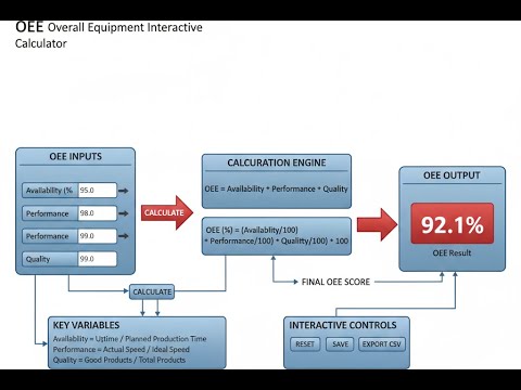
OEE Overall Equipment Effectiveness Interactive Calculator
Watch how availability, performance, and quality multiply together to determine your true productive efficiency. Adjust each factor to see immediate impact on overall equipment effectiveness and understand why even small losses compound dramatically.
OVERALL OEE
70.1%
HIDDEN CAPACITY
42.7%
TOTAL LOSSES
29.9%
CLASS RATING
FAIR
FIRGELLI Automations — Interactive Engineering Calculators
Formulas & Equations
Simple Example
A machine runs a 480-minute shift, loses 60 minutes to downtime (run time = 420 min), produces 1,000 parts at a 24-second ideal cycle time, and 950 of those parts pass quality.
- Availability = 420 / 480 = 87.5%
- Performance = (1,000 × 24 / 60) / 420 = 400 / 420 = 95.2%
- Quality = 950 / 1,000 = 95.0%
- OEE = 0.875 × 0.952 × 0.950 = 79.2%
Use the formula below to calculate Overall Equipment Effectiveness.
Overall Equipment Effectiveness (OEE)
OEE = Availability × Performance × Quality
Use the formula below to calculate Availability.
Availability
Availability = (Run Time / Planned Production Time) × 100%
Run Time = Planned Production Time - Downtime
Where:
Planned Production Time = Total time equipment is scheduled to produce (minutes)
Downtime = All unplanned stops and breakdowns (minutes)
Run Time = Actual operating time (minutes)
Use the formula below to calculate Performance.
Performance
Performance = (Ideal Cycle Time × Total Count) / Run Time × 100%
Where:
Ideal Cycle Time = Fastest possible time to manufacture one part under optimal conditions (seconds per unit)
Total Count = Total parts produced including rejects (units)
Run Time = Actual operating time converted to seconds for calculation
Use the formula below to calculate Quality Rate.
Quality
Quality = (Good Count / Total Count) × 100%
Where:
Good Count = Parts meeting quality specifications (units)
Total Count = Total parts produced including rejects (units)
Use the formula below to calculate Required Production Time.
Required Production Time
Required Time = (Target Quantity × Ideal Cycle Time) / Target OEE
Where:
Target Quantity = Desired number of good parts (units)
Ideal Cycle Time = Time per unit at design speed (seconds or minutes)
Target OEE = Expected efficiency as decimal (0.85 for 85%)
Theory & Engineering Applications
The Six Big Losses Framework
OEE emerged from Total Productive Maintenance (TPM) methodology in the 1960s, developed by Seiichi Nakajima at the Japan Institute of Plant Maintenance. The metric quantifies manufacturing inefficiency through three multiplied factors, each addressing two of the Six Big Losses: Availability captures planned stops and unplanned downtime; Performance measures speed losses and minor stops; Quality accounts for startup rejects and production defects. This multiplicative relationship means even modest losses compound dramatically—a machine running at 90% availability, 90% performance, and 90% quality achieves only 72.9% OEE, not the intuitive 90%.
The non-obvious insight that distinguishes OEE from simpler metrics is its ability to reveal hidden capacity without capital investment. A facility operating at 60% OEE theoretically possesses 67% more capacity than currently utilized (100/60 = 1.67). This realization shifts improvement focus from purchasing additional equipment to optimizing existing assets. However, OEE's multiplicative nature creates a critical limitation: improving the lowest-performing factor yields disproportionate returns, while chasing incremental gains in already-strong areas produces minimal OEE improvement. A production line at 95% availability, 70% performance, and 98% quality benefits far more from performance improvements than further availability optimization.
Availability: The Foundation Metric
Availability measures the percentage of scheduled production time that equipment actually operates. Planned production time excludes scheduled maintenance and known downtime, creating a baseline against which actual performance is measured. The critical distinction between planned stops (excluded from planned production time) and unplanned stops (counted as downtime) often creates measurement debates. Best practice defines planned stops as preventive maintenance scheduled at least 24 hours in advance with documented procedures, while all other interruptions constitute downtime regardless of cause or duration.
Equipment breakdowns dominate downtime in most facilities, but changeovers between product runs frequently contribute equal or greater losses. A packaging line requiring 45 minutes to switch between container sizes loses 7.5 hours per day with ten changeovers, equivalent to nearly one full shift. Single-Minute Exchange of Die (SMED) methodology specifically targets changeover reduction, with world-class facilities achieving changeovers in under 10 minutes for complex equipment. The economic justification for changeover reduction becomes clear when calculating opportunity cost: at 60 units per minute and $50 gross profit per unit, each minute of changeover represents $3,000 in lost margin.
Performance: Speed Loss Quantification
Performance compares actual production rate to ideal cycle time—the theoretical fastest rate achievable under optimal conditions with qualified operators, perfect materials, and no interruptions. Ideal cycle time typically comes from equipment specifications or engineering studies, not historical averages which already embed inefficiencies. Many organizations mistakenly use "budgeted" or "standard" cycle times that incorporate historical losses, artificially inflating performance scores while masking improvement opportunities.
Minor stops under five minutes often escape documentation but cumulatively devastate performance. A bottling line experiencing two-minute stops every ten minutes operates at only 80% of rated speed, yet these microstoppages rarely trigger formal downtime recording. Modern data acquisition systems detect these events through cycle time variance analysis, revealing that minor stops frequently exceed major breakdown losses in total impact. The distinction matters because countermeasures differ: major breakdowns require maintenance intervention, while minor stops typically stem from operational issues like sensor misalignment, inconsistent material supply, or operator technique variation.
Quality: First Pass Yield Integration
Quality rate measures the percentage of produced parts meeting specifications without rework. Unlike availability and performance which address time losses, quality captures value destruction—material, energy, and labor consumed to produce unmarketable output. The distinction between rejects (parts scrapped) and rework (parts requiring additional processing) creates measurement complexity. Best practice counts rework parts as rejects in initial OEE calculation, then tracks rework recovery separately to quantify the full cost of quality failures including additional processing time and labor.
Startup rejects during equipment changeovers disproportionately impact OEE in high-mix environments. A production line averaging 5% steady-state defects might experience 20% reject rates during the first 50 units after changeover. With frequent product switches, these startup losses can double overall scrap rates. Leading manufacturers implement "golden run" standards—validated changeover procedures ensuring first-part-correct startup—reducing startup rejects to match steady-state performance. The economic impact extends beyond material waste: high scrap rates during startup encourage longer production runs to amortize startup losses, increasing inventory carrying costs and reducing scheduling flexibility.
World-Class OEE Benchmarks by Industry
Automotive stamping operations typically achieve 85-90% OEE through highly automated processes with predictable cycle times and minimal changeovers. Pharmaceutical tablet coating reaches 70-75% OEE despite stringent quality requirements, with performance losses from coating uniformity validation limiting maximum rates. Food processing varies dramatically: continuous operations like dairy processing exceed 90% OEE, while batch processes with extensive cleaning requirements struggle to reach 60%. Semiconductor fabrication achieves 80-85% OEE on critical process tools through predictive maintenance and automated material handling, but older facilities with manual intervention average 65-70%.
These industry variations reflect fundamental process characteristics: continuous flow operations inherently achieve higher OEE than batch processes, automated equipment outperforms manual operations, and simple products exceed complex multi-stage assemblies. Understanding these structural differences prevents unrealistic benchmarking—a job shop producing custom components cannot match a dedicated assembly line's OEE scores. Instead, progressive organizations track OEE improvement rate as the key metric, targeting 5-10 percentage point gains annually through systematic loss reduction rather than comparing absolute scores across incompatible operations.
Fully Worked Numerical Example
Scenario: A metal stamping press operates a single shift from 7:00 AM to 3:30 PM (480 minutes planned production time). During the shift, the press experiences two breakdowns totaling 37 minutes and four changeovers totaling 68 minutes. The ideal cycle time for the current part is 8.2 seconds per piece. The press produces 2,847 total parts, of which 2,691 meet quality specifications. Calculate complete OEE and identify the primary loss category.
Given Information:
- Planned Production Time = 480 minutes
- Breakdown Downtime = 37 minutes
- Changeover Time = 68 minutes
- Total Downtime = 37 + 68 = 105 minutes
- Ideal Cycle Time = 8.2 seconds per piece
- Total Parts Produced = 2,847 pieces
- Good Parts = 2,691 pieces
Step 1: Calculate Run Time
Run Time = Planned Production Time - Total Downtime
Run Time = 480 minutes - 105 minutes = 375 minutes
Step 2: Calculate Availability
Availability = (Run Time / Planned Production Time) × 100%
Availability = (375 / 480) × 100% = 78.125%
Step 3: Calculate Performance
First, convert run time to seconds: 375 minutes × 60 = 22,500 seconds
Ideal Production Time = Total Parts × Ideal Cycle Time
Ideal Production Time = 2,847 parts × 8.2 seconds/part = 23,345.4 seconds
Performance = (Ideal Production Time / Run Time) × 100%
Performance = (23,345.4 / 22,500) × 100% = 103.76%
Performance Validation: The calculated performance exceeds 100%, which is theoretically impossible. This indicates the ideal cycle time (8.2 seconds) is incorrectly specified—the press is actually operating faster than the stated "ideal" rate. This common error occurs when ideal cycle time is set conservatively. For calculation purposes, we cap performance at 100% and note that ideal cycle time requires re-validation through time studies. Using 100% performance for final OEE calculation represents the maximum possible performance contribution.
Step 4: Calculate Quality
Quality = (Good Parts / Total Parts) × 100%
Quality = (2,691 / 2,847) × 100% = 94.522%
Step 5: Calculate Overall OEE
OEE = Availability × Performance × Quality
Using capped performance: OEE = 0.78125 × 1.00 × 0.94522
OEE = 0.7385 = 73.85%
Step 6: Identify Loss Analysis
Availability Loss = 100% - 78.125% = 21.875%
Performance Loss = 100% - 100% = 0% (after capping, but indicates measurement error)
Quality Loss = 100% - 94.522% = 5.478%
Conclusion: The press operates at 73.85% OEE, solidly in the "industry average" range (60-84%). Availability represents the primary loss at 21.875%, driven by 105 minutes of downtime—22% of planned production time. The 68-minute changeover contribution (64.8% of total downtime) suggests SMED methodology could deliver significant OEE improvement. The performance exceeding 100% indicates equipment capability exceeds documented ideal cycle time, requiring engineering review to establish accurate baseline. Quality losses of 5.5% are relatively minor but represent 156 rejected parts worth further investigation to determine if startup rejects or process drift drives the defect rate. Prioritizing changeover reduction offers the highest ROI, potentially recovering 10-15 OEE points through structured improvement.
For more specialized engineering calculations, visit our comprehensive engineering calculator library.
Practical Applications
Scenario: Justifying Automation Investment
Marcus, a manufacturing engineer at an automotive tier-1 supplier, needs to justify a $2.3M automated inspection system to replace manual quality checks on transmission components. His current manual process achieves 68% OEE: 88% availability (frequent inspector breaks and shift changes), 82% performance (inconsistent inspection speed), and 94% quality (occasional inspection errors). He uses the OEE calculator to model the automated system's projected performance—95% availability, 98% performance, 99.5% quality—yielding 92.6% OEE. The 24.6 percentage point improvement translates to 36% capacity increase from the same equipment footprint. At 12,000 parts per day and $18 gross margin per part, the additional capacity generates $2.4M annual profit, providing a one-year payback. The calculator's required production time mode confirms the facility can meet a new contract requiring 15,000 daily parts within existing shift structures at 92% OEE, but would require overtime at current 68% efficiency.
Scenario: Diagnosing Performance Loss on Packaging Line
Jennifer, a continuous improvement manager at a food processing plant, investigates why her bottling line's OEE dropped from 79% to 71% over six weeks despite no major equipment failures. She uses the calculator's component modes to isolate the problem: availability remained stable at 85%, quality actually improved slightly to 96%, but performance declined from 87% to 87%. Wait—87% to 87% shows no change, yet OEE dropped 8 points. She recalculates using actual production counts and discovers the ideal cycle time in the system (changed during a recent software update) increased from 1.8 to 2.1 seconds per bottle, masking a real performance decline. Calculating performance with the original 1.8-second ideal cycle time reveals actual performance dropped to 74%. Root cause investigation identifies worn timing belts causing intermittent slowdowns. The calculator helped cut through misleading data to identify a mechanical issue that would have worsened into catastrophic failure, preventing an estimated $47,000 weekend breakdown with rush delivery of replacement components.
Scenario: Production Planning for New Product Launch
Aisha, a production planner at a consumer electronics manufacturer, must schedule production for a new wireless charger launching in 12 weeks. Marketing demands 250,000 units for launch inventory. Her injection molding line produces the charger housing with a 23-second ideal cycle time per part and historical 76% OEE across similar products. Using the calculator's required production time mode, she calculates needing 1,208 hours (23 seconds × 250,000 parts / 0.76 / 3,600 seconds per hour). With two shifts of 8 hours each available five days weekly, she has 960 hours over 12 weeks—insufficient by 248 hours. Rather than authorize expensive overtime immediately, she models scenarios: achieving 85% OEE through pre-launch equipment upgrades reduces required time to 1,081 hours, fitting within normal shifts with buffer time. She also discovers that reducing the 23-second cycle time by just 1.5 seconds through mold cooling optimization at 76% OEE eliminates the time deficit. The calculator transformed an apparent overtime crisis into actionable improvement targets, ultimately saving $68,000 in premium labor costs while building organizational capability.
Frequently Asked Questions
What is a "good" OEE score and how does it vary by industry? +
Should planned maintenance be included in OEE calculations? +
How do I determine the correct ideal cycle time for my equipment? +
Can OEE be calculated for manual assembly operations? +
What data collection frequency is needed for accurate OEE tracking? +
How does OEE relate to Overall Labor Effectiveness (OLE)? +
Free Engineering Calculators
Explore our complete library of free engineering and physics calculators.
Browse All Calculators →🔗 Explore More Free Engineering Calculators
About the Author
Robbie Dickson — Chief Engineer & Founder, FIRGELLI Automations
Robbie Dickson brings over two decades of engineering expertise to FIRGELLI Automations. With a distinguished career at Rolls-Royce, BMW, and Ford, he has deep expertise in mechanical systems, actuator technology, and precision engineering.
Need to implement these calculations?
Explore the precision-engineered motion control solutions used by top engineers.


