Wave Velocity Interactive Calculator

The Wave Velocity Interactive Calculator computes the speed at which wave disturbances propagate through different media, from electromagnetic radiation in vacuum to mechanical waves in strings, fluids, and solids. Wave velocity determines everything from fiber optic data transmission rates to seismic wave arrival times used in earthquake location, making it fundamental to telecommunications engineering, acoustics, geophysics, and materials testing. This calculator handles frequency-wavelength relationships, tension-based string velocities, and medium-dependent propagation speeds across multiple physical contexts.

📐 Browse all free engineering calculators

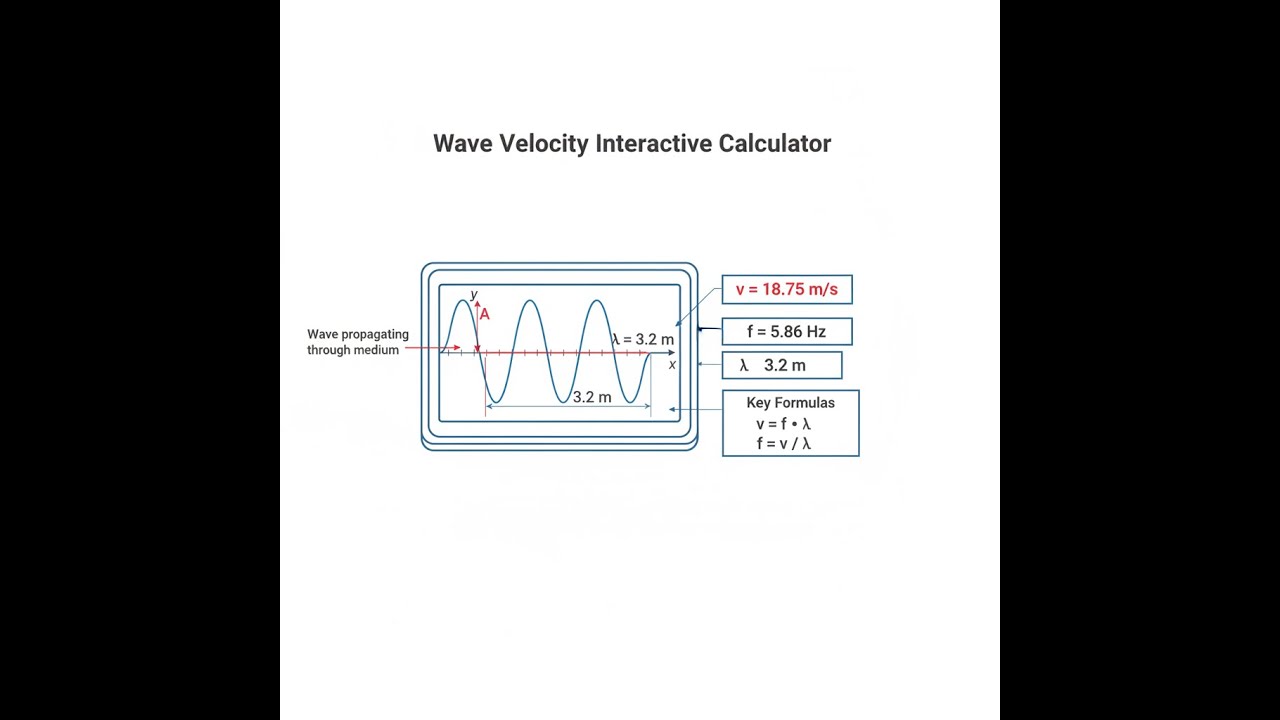
Wave Propagation Diagram

Interactive Wave Velocity Calculator

Wave Velocity Equations

Theory & Practical Applications

Fundamental Physics of Wave Propagation

Wave velocity represents the speed at which a disturbance propagates through a medium, fundamentally distinct from the velocity of individual particles within that medium. For mechanical waves, propagation depends on two competing factors: the restoring force that returns displaced material to equilibrium (represented by elastic moduli or tension) and the inertia that resists acceleration (represented by density or linear mass density). This creates the universal pattern v ∝ √(stiffness/inertia) seen across all mechanical wave types.

The frequency-wavelength relationship v = fλ is deceptively simple but reveals critical physics. For a given medium with fixed wave velocity, frequency and wavelength are inversely coupled — doubling frequency halves wavelength. This constraint governs everything from ultrasonic testing probe design (where higher frequencies provide better spatial resolution via shorter wavelengths) to architectural acoustics (where low-frequency sound with its long wavelength more easily diffracts around obstacles). The product remains constant only if the medium properties remain unchanged, which fails at interfaces, in dispersive media, or when wave amplitude becomes large enough to induce nonlinear effects.

String Wave Mechanics and Musical Instruments

The string wave equation v = √(T/μ) governs vibrating strings in musical instruments from guitar strings to piano wires. Linear mass density μ = m/L combines material density with cross-sectional geometry — a steel string and nylon string of identical diameter have drastically different μ values, producing different fundamental frequencies at the same tension. Instrument designers manipulate this relationship: guitar strings are tuned by adjusting tension T while maintaining fixed μ and length L, whereas selecting thicker strings increases μ to reach lower pitches without reducing tension to mechanically unstable levels.

Critical tension limits arise from material yield strength. A steel string with 1 mm diameter and 650 mm length has linear density approximately 0.00502 kg/m. To achieve A440 (440 Hz) with fundamental mode wavelength λ = 2L = 1.3 m requires v = 440 × 1.3 = 572 m/s, demanding tension T = μv² = 0.00502 × (572)² = 1641 N. This produces stress σ = T/A = 1641/(π × 0.0005²) ≈ 2.09 GPa, approaching the 2.5 GPa yield strength of music wire — explaining why high-tension instruments like pianos use multiple strings per note and require robust engineering of the structural frame that sustains cumulative tensions exceeding 20,000 N.

Sound Propagation in Fluids and Gases

Sound velocity in fluids v = √(K/ρ) depends on bulk modulus K, which measures volumetric compressibility. Water has K ≈ 2.2 × 10⁹ Pa and ρ = 1000 kg/m³, yielding v = √(2.2×10⁹/1000) = 1483 m/s. Air at 20°C has effective K ≈ 1.42 × 10⁵ Pa and ρ = 1.204 kg/m³, giving v = 343 m/s. The five-fold difference between underwater and aerial sound speeds profoundly affects sonar systems, marine mammal communication, and underwater construction monitoring.

Temperature dependence enters through density variation. For ideal gases, v = √(γRT/M) where γ is the heat capacity ratio, R the gas constant, T absolute temperature, and M molar mass. Air sound speed increases approximately 0.6 m/s per degree Celsius, creating atmospheric refraction that bends sound rays. This explains why sound carries farther on cold nights (temperature inversions trap sound near the ground) and why accurate acoustic ranging requires temperature correction. Humidity also affects M by replacing heavier N₂ and O₂ molecules with lighter H₂O, increasing velocity by up to 4 m/s in saturated air — non-negligible for precision acoustic measurements.

Elastic Waves in Solids and Seismic Applications

Solids support multiple wave types: longitudinal (P-waves), transverse (S-waves), and surface waves (Rayleigh, Love). Longitudinal velocity v_P = √(E/ρ) uses Young's modulus for thin rod approximation, but in bulk solids the full expression involves both bulk modulus K and shear modulus G: v_P = √[(K + 4G/3)/ρ]. Steel with E = 200 GPa and ρ = 7850 kg/m³ has v_P ≈ 5048 m/s. Shear waves travel slower: v_S = √(G/ρ) ≈ 3150 m/s for steel.

Seismology exploits the P-wave/S-wave arrival time difference to locate earthquakes. P-waves arrive first (primary), followed by S-waves (secondary). If a seismic station records a 12-second interval between P and S arrivals, and regional velocities are v_P = 6.8 km/s and v_S = 3.9 km/s in crustal rock, the distance d satisfies: d/v_S - d/v_P = 12 s. Solving: d(1/3900 - 1/6800) = 12, yielding d/3900 - d/6800 = 12. This gives d(6800 - 3900)/(3900 × 6800) = 12, so d × 2900/26,520,000 = 12, resulting in d = 109.7 km. Three stations provide triangulation for epicenter location, with depth requiring additional phase analysis.

Worked Example: Ultrasonic Testing Transducer Design

Problem: An ultrasonic testing (UT) technician needs to inspect a steel pressure vessel for internal cracks using a 5 MHz longitudinal wave transducer. The steel has density ρ = 7850 kg/m³ and Young's modulus E = 207 GPa. The transducer resolution is approximately half the wavelength. Calculate: (a) the longitudinal wave velocity in the steel, (b) the wavelength of the 5 MHz ultrasound, (c) the minimum detectable crack size, (d) the time for the ultrasound to travel through a 150 mm thick vessel wall and return, and (e) the frequency required to detect 0.25 mm cracks.

Solution:

Part (a): Longitudinal wave velocity in steel:

v = √(E/ρ) = √(207 × 10⁹ Pa / 7850 kg/m³)

v = √(26,369,426.75 m²/s²) = 5135.2 m/s

Part (b): Wavelength at 5 MHz:

λ = v/f = 5135.2 m/s / (5 × 10⁶ Hz)

λ = 1.0270 × 10⁻³ m = 1.027 mm

Part (c): Minimum detectable crack size (λ/2 resolution limit):

Minimum crack size = λ/2 = 1.027 mm / 2 = 0.514 mm

This transducer can detect cracks approximately 0.5 mm or larger.

Part (d): Round-trip travel time through 150 mm wall:

Total distance = 2 × 150 mm = 300 mm = 0.300 m

Time = distance/velocity = 0.300 m / 5135.2 m/s

Time = 5.842 × 10⁻⁵ s = 58.42 μs

The echo returns after approximately 58.4 microseconds.

Part (e): Frequency for 0.25 mm crack detection:

Required wavelength: λ = 2 × 0.25 mm = 0.50 mm = 5.0 × 10⁻⁴ m

Required frequency: f = v/λ = 5135.2 m/s / (5.0 × 10⁻⁴ m)

f = 10.27 × 10⁶ Hz = 10.27 MHz

A 10 MHz or higher transducer is needed for 0.25 mm resolution.

Engineering Implications: Higher frequencies provide better spatial resolution but suffer greater attenuation in the material. The UT technician must balance resolution requirements against penetration depth. For thick-walled pressure vessels, 5 MHz represents a practical compromise. Near-surface defects might justify 10-15 MHz probes, while very thick sections may require dropping to 2.25 MHz. The 58.4 μs echo delay allows time-of-flight measurement, enabling the simultaneous determination of both defect presence and wall thickness — critical for corrosion monitoring in petrochemical facilities.

Dispersion and Frequency-Dependent Velocity

The fundamental equation v = fλ assumes non-dispersive propagation where all frequencies travel at identical velocity. Real media often exhibit dispersion, where wave velocity depends on frequency. Ocean surface waves demonstrate strong dispersion: deep-water phase velocity v_phase = √(gλ/2π) increases with wavelength, causing long-period swell to outrun shorter wind waves generated by the same storm. Group velocity v_group = dω/dk describes energy transport and equals v_phase/2 for deep-water gravity waves, explaining why wave packets travel at half the phase velocity of individual crests.

Optical fibers exhibit chromatic dispersion because the refractive index n(λ) varies with wavelength, causing different wavelengths to propagate at different velocities v = c/n. This pulse-spreading limits data transmission rates. Single-mode fibers operating near the 1550 nm telecommunications window are engineered for zero-dispersion wavelength, where d²n/dλ² = 0, enabling 100 Gb/s transmission over hundreds of kilometers. Without dispersion compensation, a 10 ps pulse launched into standard single-mode fiber (dispersion parameter D ≈ 17 ps/(nm·km)) broadens by Δt = D × Δλ × L. For Δλ = 0.1 nm spectral width over L = 50 km: Δt = 17 × 0.1 × 50 = 85 ps, increasing pulse duration nearly tenfold.

Industrial Applications and Measurement Techniques

Wave velocity measurements enable non-destructive material characterization. Measuring longitudinal and shear wave velocities in a sample allows determination of elastic constants: E = ρv_P²[(1+ν)(1-2ν)/(1-ν)] and G = ρv_S², where Poisson's ratio ν = (v_P²/v_S² - 2)/(2v_P²/v_S² - 2). This technique evaluates concrete curing (velocity increases as hydration progresses), detects frost damage in pavement (velocity drops when pore water freezes), and assesses fatigue damage in aerospace components (microcrack accumulation reduces effective modulus).

Acoustic flow metering exploits velocity differences for upstream versus downstream sound propagation. In a fluid flowing at velocity u, sound traveling at angle θ to the flow has effective velocity v ± u·cos(θ). Transit time difference Δt between opposed transducers separated by distance L allows flow velocity calculation: u = (L/2·cos(θ)) × (Δt/t₁t₂), where t₁ and t₂ are individual transit times. For water (v = 1483 m/s) flowing at 2.5 m/s with transducers at 45° and L = 200 mm: the transit time difference is approximately Δt = 2Lu·cos(θ)/v² = 2 × 0.2 × 2.5 × 0.707 / 1483² ≈ 0.32 μs. Precision timing electronics resolve nanosecond differences, enabling 0.5% flow measurement accuracy.

For additional wave and electromagnetic calculations, visit the engineering calculator hub.

Frequently Asked Questions