Lensmakers Equation Interactive Calculator

The Lensmaker's Equation calculates the focal length of a thin lens based on its curvature radii and refractive index. This fundamental relationship enables optical engineers to design precision imaging systems, from microscope objectives to camera lenses, by predicting how light converges or diverges through glass elements. Understanding this equation is essential for anyone working in photonics, machine vision, laser systems, or optical instrumentation where exact focal control determines system performance.

📐 Browse all free engineering calculators

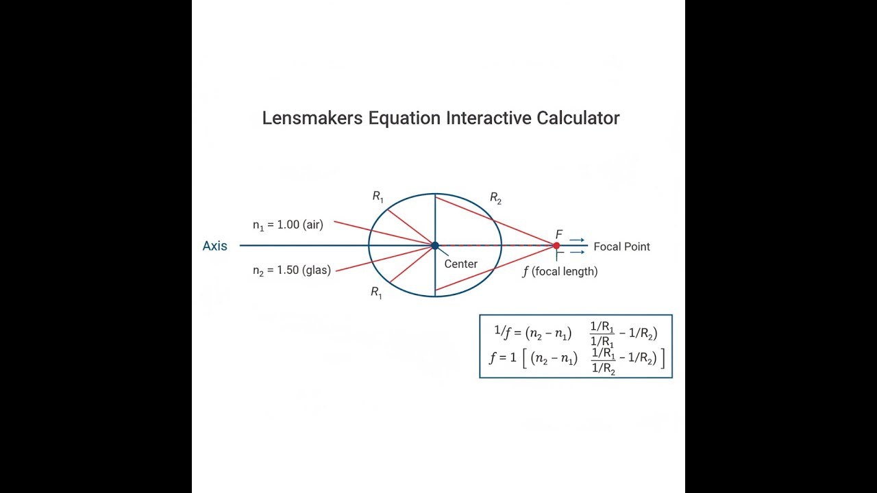
Lens Geometry Diagram

Interactive Lensmaker's Equation Calculator

Governing Equations

Theory & Practical Applications

Fundamental Principles of Lens Refraction

The Lensmaker's Equation derives from Snell's law applied sequentially at both refracting surfaces of a thin lens. When parallel light enters a lens, each surface acts as a refracting interface where the change in optical medium causes ray bending. The equation assumes paraxial conditions—rays travel close to and nearly parallel to the optical axis—which breaks down for wide-angle systems or high numerical apertures. Real lens design must account for spherical aberration when aperture angles exceed approximately 10°, at which point ray-tracing software becomes essential.

A critical but often overlooked aspect is the sign convention for radii of curvature. In standard optical engineering notation, R₁ is positive when the first surface is convex toward the incoming light (center of curvature lies beyond the surface), and negative when concave. For R₂, the sign reverses because we measure from the exit side—positive means the center of curvature is to the left of the surface (concave from the entry perspective). This asymmetry causes frequent calculation errors. A symmetric biconvex lens typically has R₁ positive and R₂ negative, both with equal magnitudes.

Material Selection and Refractive Index Engineering

The factor (n₂/n₁ - 1) governs how strongly a lens bends light. Crown glass with n = 1.52 in air (n₁ = 1.00) provides moderate refraction suitable for general optics. High-index materials like dense flint glass (n = 1.72) or specialized polymers enable shorter focal lengths from gentler curvatures, reducing manufacturing difficulty and spherical aberration. However, high-index glasses often exhibit greater chromatic dispersion, causing color-dependent focal shifts. Achromatic doublets combat this by pairing crown and flint elements with opposite dispersions but matched powers at design wavelengths.

Immersion systems deliberately use n₁ > 1 by placing oil (n ≈ 1.52) between lens and specimen, as in microscopy. This reduces the n₂/n₁ ratio, requiring stronger curvatures to achieve the same focal length, but dramatically increases numerical aperture and resolution. The Lensmaker's Equation shows that halving the refractive index contrast doubles the required curvature term (1/R₁ - 1/R₂) for constant focal length—a fundamental trade-off in optical design.

Multi-Element System Design

Real optical instruments rarely use single lenses. Camera objectives may contain 10+ elements, each calculated using the Lensmaker's Equation as a starting approximation before iterative optimization. When two thin lenses are separated by distance d, the system focal length becomes f_total = (f₁f₂)/(f₁ + f₂ - d). At d = 0 (lenses in contact), this reduces to the additive power formula P_total = P₁ + P₂. This additivity makes diopters convenient for prescription eyeglasses where multiple corrections stack.

Telephoto designs exploit negative-positive lens combinations to achieve long focal lengths in compact packages. A positive front element with f₁ = +200 mm paired with a rear negative element at f₂ = -100 mm yields f_total = +200 mm, but the back focal distance (image plane to rear lens) can be just 50 mm—half the effective focal length. This geometry explains how 300 mm telephoto camera lenses fit into 150 mm barrels.

Worked Engineering Example: Laser Beam Expander Design

An industrial laser system requires expanding a 2 mm diameter beam to 10 mm for reduced intensity at the workpiece. Design a Galilean beam expander using BK7 glass (n = 1.5168 at 632.8 nm HeNe wavelength) with a 5× magnification ratio.

Step 1: Determine focal length relationship. For a Galilean telescope (afocal system), the magnification M = -f₂/f₁ where f₁ is the negative input lens and f₂ is the positive output lens. For M = 5, we need f₂ = -5f₁. Choose f₁ = -40 mm, giving f₂ = +200 mm. The negative lens diverges the beam, and the positive lens collimates it at larger diameter.

Step 2: Design the input diverging lens. Select a plano-concave geometry with the flat surface (R₁ = ∞) facing the laser and curved surface facing outward. The Lensmaker's Equation becomes:

1/(-40) = (1.5168/1.00 - 1)(1/∞ - 1/R₂)
-0.025 = 0.5168(-1/R₂)
R₂ = 0.5168/0.025 = 20.672 mm

The concave surface requires R₂ = +20.67 mm (positive because center of curvature is to the left from the exit side). Physically, this is a 41.34 mm diameter sphere creating a concave surface with -20.67 mm radius from the entry perspective.

Step 3: Design the output converging lens. For the f₂ = +200 mm positive lens, use a symmetric biconvex form (R₁ = -R₂) for minimal spherical aberration:

1/200 = (1.5168/1.00 - 1)(1/R₁ - 1/R₂)
0.005 = 0.5168(2/R₁) for symmetric lens
R₁ = 2(0.5168)/0.005 = 206.72 mm

This requires R₁ = +206.72 mm and R₂ = -206.72 mm. Each surface is a section of a 413.44 mm diameter sphere.

Step 4: Verify system performance. Lens separation d = f₁ + f₂ = -40 + 200 = 160 mm for afocal operation. Input beam divergence angle after first lens: θ₁ = beam_diameter/(2f₁) = 2/(2×40) = 0.025 rad. After second lens, output angle θ₂ = beam_diameter/(2f₂) = 10/(2×200) = 0.025 rad. The angles match, confirming afocal alignment and 5× expansion.

Step 5: Manufacturing tolerances. For λ/10 wavefront error at 632.8 nm, surface radius tolerance is approximately ±0.5% or ±1 mm on R₁ for the positive lens. The negative lens, with tighter curvature, requires ±0.1 mm on R₂. Centering tolerance between lenses must be within 50 μm to prevent beam deviation exceeding 0.1 mrad. These specifications determine manufacturing cost—the plano-concave element is significantly cheaper to produce than the large-radius biconvex element.

Industrial Applications Across Sectors

Machine vision systems for quality inspection rely on precision lenses designed via the Lensmaker's Equation to achieve diffraction-limited resolution at working distances of 100-500 mm. A typical 25 mm focal length lens for a 2/3" sensor might use four elements totaling 12 optical surfaces, each radius calculated initially from thin lens equations then refined through Zemax optimization. Telecentricity requirements (parallel chief rays) often necessitate symmetric doublets with matched but opposite powers, achievable only through careful radius selection.

Fiber optic collimators use gradient-index (GRIN) rod lenses or aspheric molded elements to couple laser diodes into single-mode fibers. The required numerical aperture of 0.1-0.14 translates to focal lengths of 2-4 mm for typical 9 μm core fibers. At these scales, the thin lens approximation breaks down, but the Lensmaker's Equation still guides initial curvature selection before full ray-trace analysis. Aspheric departures from spherical surfaces can reduce spot size by 60% compared to purely spherical designs.

Ophthalmic lens manufacturing uses negative meniscus geometries (both surfaces concave toward the eye) for myopia correction. A -3.00 D prescription lens in CR-39 plastic (n = 1.498) with base curve R₁ = -200 mm requires R₂ calculated from 1/f = -3.00 m⁻¹ = (1.498 - 1)(1/(-200×10⁻³) - 1/R₂). Solving gives R₂ = -0.118 m or -118 mm. The meniscus shape reduces oblique aberrations compared to plano-concave alternatives, critical for peripheral vision quality.

Thermal and Environmental Considerations

Glass refractive index varies with temperature at rates of dn/dT ≈ +1 to +10 × 10⁻⁶ K⁻¹ for most optical glasses. A BK7 lens with n = 1.5168 at 20°C shifts to n = 1.5200 at 100°C, changing focal length by approximately 0.2%. For a 500 mm focal length telescope objective, this 1 mm shift can defocus stellar images. Athermal lens designs pair positive and negative elements with opposite dn/dT coefficients, using the Lensmaker's Equation to balance thermal focal shifts across temperature ranges of -40°C to +80°C in aerospace applications.

Frequently Asked Questions