Friction Factor Interactive Calculator

If you’re laying out a piping system and don’t have decent friction data, you’re basically making educated guesses for pump size, expected pressure drop, and how much flow you'll really get — and those guesses add up quickly. The calculator below lets you work out the Darcy-Weisbach friction factor, factoring in Reynolds number, pipe roughness, size, and your specific fluid — with six core calculation options. Getting friction factors about right is a basic requirement in things like HVAC, factory hydraulics, and water supply lines, since pressure losses hit efficiency and actuator performance directly. On this page, you’ll get the relevant equations, a real-world worked example, basic flow regime theory, and practical notes on odd cases such as pipe aging and non-Newtonian fluids.

What is Friction Factor?

Friction factor is a dimensionless value that tells you how much a fluid resists moving through a pipe. Larger numbers mean you lose more pressure to friction along the way, so the pump (or actuator) needs to work harder to keep things moving.

Simple Explanation

Pushing water through a smooth hose is much easier than through a rough concrete pipe — the friction factor is just a way to give a useful number to that extra effort. It goes up with a rougher surface or faster flow, but the shear between pipe wall and fluid depends on whether the flow is orderly (laminar) or all mixed up (turbulent). The friction factor gives you a direct estimate of the pressure loss per length.

📐 Browse all 1000+ Interactive Calculators

Diagram

Friction Factor Interactive Calculator

How to Use This Calculator

1. Pick a calculation mode — laminar, turbulent (Colebrook-White), Swamee-Jain, Haaland, Reynolds number from flow rate, or pressure drop.
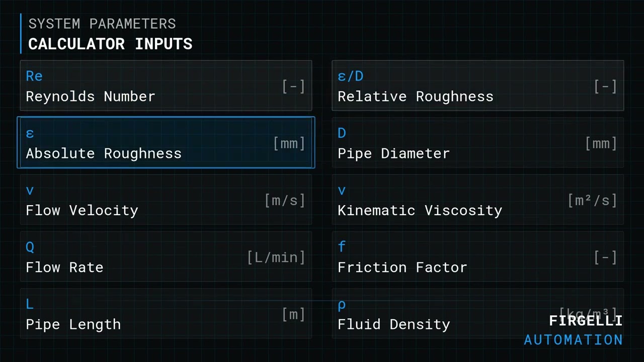
2. Fill in whatever inputs the calculator asks for — that might be Reynolds number, diameter, roughness, velocity, density, or viscosity, depending on the mode.
3. Check units: diameter and roughness in mm, velocity in m/s, flow rate in L/min, viscosity in m²/s, density in kg/m³.
4. Click Calculate and check your result.

📹 Video Walkthrough — How to Use This Calculator

Equations

Simple Example

Laminar flow in a hydraulic line: Re = 500, pipe diameter = 10 mm, fluid is water.

• Flow regime: Laminar (Re < 2300) ✓
• Friction factor: f = 64 / 500 = 0.128
• At v = 1 m/s, L = 10 m, ρ = 1000 kg/m³: ΔP = 0.128 × (10/0.01) × (1000 × 1² / 2) = 64,000 Pa = 64 kPa

Theory & Practical Applications

Fundamental Flow Resistance Physics

The Darcy-Weisbach friction factor measures how much the pipe wall and flow characteristics slow things down in a round pipe. Unlike the Hazen-Williams coefficient, it's rooted in the actual physics. When Re < 2300, the friction factor comes right out of solving the flow equations for steady laminar flow in a round pipe — you get f = 64/Re, but only if you have fully developed, Newtonian flow in a horizontal, round pipe.

For Re above about 4000, you enter the turbulent regime. Here, most of the flow energy goes into chaotic mixing, but a thin layer near the wall is still controlled by viscosity. If the wall is rough, those bumps start to stick out through the viscous layer once a certain threshold is crossed. At that point, roughness dominates, and friction factor stops depending on Reynolds number — it’s mainly a function of ε/D only. The Colebrook-White equation handles this by combining the effects of roughness and turbulence, but you have to use iteration to solve it. If you want something faster, approximations like Swamee-Jain and Haaland get you close, mainly for quick or repetitive calculations where perfect precision isn’t worth the time.

Industrial Applications and Material Selection

Friction factor math ties directly to how big your pump needs to be. Over long pipes — pipelines for water, oil, gas — shaving down the friction factor with a cleaner or smoother pipe can save a noticeable amount on energy costs over time. Standard steel pipe is around ε = 0.045 mm, but drawn tubing is much smoother, closer to ε = 0.0015 mm. PVC and polyethylene start out smooth (about ε = 0.0015 mm) but can get much rougher as scale or biofilm builds up over years of use.

For hydraulic setups, especially systems using actuators to control position, you need a good grip on pressure losses or you can’t predict force accurately. Narrow pipes (6 mm bore) can lose 50-150 kPa pressure for every meter at typical flows — that adds up, even against 20 MPa system pressure. For micro-hydraulics (sub-mm bores), flow usually stays laminar, so you can just stick with f = 64/Re — there’s no need to use more complicated models.

Moody Diagram and Flow Regime Transitions

The Moody diagram is a tool for quickly seeing how friction factor depends on Reynolds number and roughness. You’ll see that in the "transition" zone between 2300 < Re < 4000, the flow is unstable: friction factor bounces around and isn’t reliable, so you usually want to avoid designing for this zone. Laminar flow can sometimes persist up to Re = 3000 if the system is very clean and undisturbed, but under real conditions, transition usually happens by Re = 2000-4000, especially if the entrance or pipe wall is rough.

For relatively smooth pipes with moderate Reynolds numbers, the Blasius formula (f = 0.316/Re^0.25) tracks friction factor pretty well between Re = 4000 and Re = 100,000. In this domain, as Reynolds number increases, the friction factor still drops — but once the pipe is fully rough, that stops, and f becomes nearly constant. Always check which regime your setup is actually in: for example, a steel pipe with D = 150 mm and ε/D = 0.0003 is on the edge between smooth and rough at Re = 50,000, so you’ll need Colebrook-White if you want it right.

Non-Circular Ducts and Hydraulic Diameter

You can extend the Darcy-Weisbach approach to non-round ducts if you use hydraulic diameter: D_h = 4A/P, where A is the cross-sectional area and P is the wetted perimeter. For a rectangle (width W and height H), D_h = 2WH/(W+H). But be careful — the friction factors for non-circular ducts aren’t always identical to what you get from circular-pipe equations, even after this substitution. For example, square ducts have about 13% higher friction factor than round pipes of the same hydraulic diameter at identical Re, mostly because you get extra mixing in the corners.

Compressibility Effects in Gas Flow

Whenever you’re designing for gas flow with more than about 10% pressure drop across the length, changing density matters. Under isothermal conditions (when heat loss or gain keeps temperature roughly constant), you end up with a quadratic relation between inlet/outlet pressures and velocity, and you have to use the speed of sound as part of your calc. In natural gas lines, expect 15-20% density drop from start to end, which — if ignored — causes you to overpredict pressure loss by 5-8%. For smaller lines or very low pressure drops, treating density as constant is usually good enough.

Worked Example: Hydraulic System for Industrial Positioning

A positioning robot driven by hydraulic actuators needs to hit a position within ±0.5 mm. The setup is:

• Hydraulic fluid: ISO VG 32 oil at 40°C (ρ = 872 kg/m³, ν = 32×10⁻⁶ m²/s)
• Supply: 8 mm ID commercial steel tube (ε = 0.045 mm)
• Pipe run: L = 4.8 m
• Required flow: Q = 3.6 L/min for the needed actuator speed
• Pump outlet pressure: 15 MPa

Part A: Reynolds number and regime

First, convert Q to m³/s:
Q = 3.6 L/min × (1 m³/1000 L) × (1 min/60 s) = 6.0×10⁻⁵ m³/s

Find velocity:
D = 8 mm = 0.008 m
A = πD²/4 = π(0.008)²/4 = 5.027×10⁻⁵ m²
v = Q/A = 6.0×10⁻⁵ / 5.027×10⁻⁵ = 1.194 m/s

Now Re:
Re = vD/ν = (1.194)(0.008)/(32×10⁻⁶) = 298.5

Result: Re = 298.5 — well below 2300, so flow is laminar.

Part B: Friction factor and pressure drop

Laminar flow:
f = 64/Re = 64/298.5 = 0.2144

Roughness (mostly irrelevant in laminar flow, but for reference):
ε/D = 0.045 mm / 8 mm = 0.00563

Darcy-Weisbach equation:
ΔP = f × (L/D) × (ρv²/2)
ΔP = 0.2144 × (4.8/0.008) × (872 × 1.194² / 2)
ΔP = 0.2144 × 600 × 621.9
ΔP = 80,000 Pa = 80 kPa

Result: 80 kPa pressure loss over 4.8 m — about 0.53% of your 15 MPa system pressure. Not usually a problem for most industrial accuracy requirements.

Part C: Actuator force at line end

P_actuator = P_pump - ΔP = 15,000 kPa - 80 kPa = 14,920 kPa

Piston area (20 mm bore):
A = π×0.01² = 3.142×10⁻⁴ m²
F = P × A = 14,920,000 Pa × 3.142×10⁻⁴ m² = 4688 N

Result: Actuator gives 4688 N force, compared to 4712 N with no line loss — roughly a 0.5% reduction. In practical positioning tasks, this is generally within normal error bands.

Part D: If you bump the flow up 50%

New flow Q = 5.4 L/min (say, fast retraction mode):
v_new = 1.194 × 1.5 = 1.791 m/s
Re_new = 298.5 × 1.5 = 447.8 (still laminar)

New friction factor: f = 64/447.8 = 0.1429

New pressure drop:
ΔP_new = f × (L/D) × (ρv_new²/2)
ΔP_new = 0.1429 × 600 × (872 × 1.791² / 2)
ΔP_new = 0.1429 × 600 × 1399.5
ΔP_new = 120,000 Pa = 120 kPa

Result: Now, pressure drop goes to 120 kPa with 50% more flow. Because you’re in laminar regime, the pressure drop scales in proportion to the velocity, so it’s still predictable. The loss is still less than 1% of total pressure; for most applications, that’s still workable.

This is why, even with small tubes and moderate pressures, you can't ignore line losses in hydraulic automation or motion systems. If you want to know what real-world actuators will do, realistic pressure loss — not just the ideal system pressure — should be considered at the design stage.

FAQ