Running a manufacturing line at full speed doesn't mean you're running it efficiently — two completely different problems that require two completely different metrics. Use this Capacity Utilization and OEE calculator to calculate how effectively your equipment and facilities are being used, using inputs for availability, performance, quality, actual output, and planned production time. These metrics matter across automotive assembly, pharmaceutical packaging, semiconductor fabrication, and any capital-intensive process where hidden losses quietly erode throughput. This page includes the full OEE and capacity utilization formulas, a worked shift-level example, theory on the six big losses framework, and a detailed FAQ.
What is OEE and Capacity Utilization?
OEE (Overall Equipment Effectiveness) is a single percentage that tells you how much of your planned production time is actually generating good parts. Capacity utilization tells you what fraction of your maximum possible output you're currently producing. Both numbers together give you the full picture of where production is being lost.
Simple Explanation
Think of OEE like a leaky bucket — even if your machine is running, time drains away through breakdowns, slow cycles, and defective parts. OEE multiplies 3 factors together (uptime, speed, and yield) to measure exactly how much of the bucket actually fills up. Capacity utilization is simpler: it just asks how much you produced versus how much you theoretically could have produced.
📐 Browse all 1000+ Interactive Calculators
How to Use This Calculator
- Select your calculation mode from the dropdown — OEE from components, capacity utilization, availability, performance, quality, or reverse target calculation.
- Enter the input values for your selected mode — percentages, unit counts, or time values in hours as prompted by the visible fields.
- Check that all values are within valid ranges (percentages between 0 and 100, time and unit values positive and non-zero).
- Click Calculate to see your result.
Visual Diagram: OEE Components and Capacity Flow

Capacity Utilization & OEE Calculator
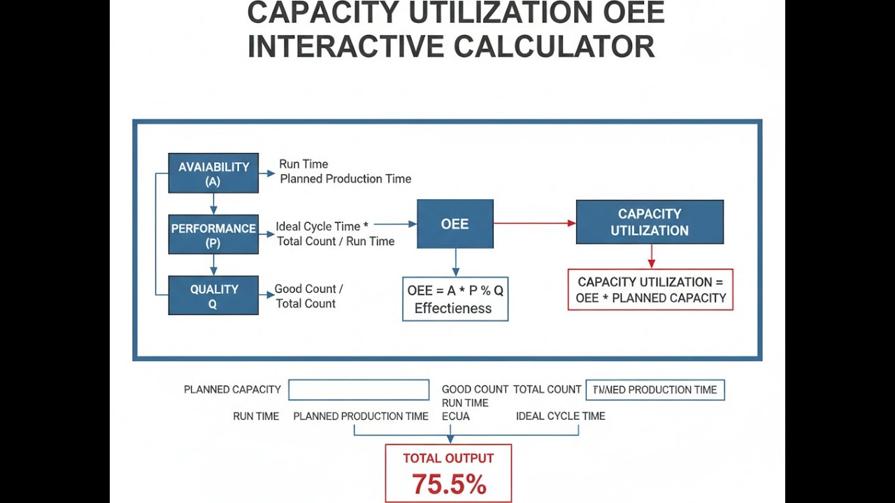
Capacity Utilization & OEE Interactive Visualizer
Watch how availability, performance, and quality factors multiply together to determine your Overall Equipment Effectiveness. See the hidden impact of minor stops and quality losses on your manufacturing throughput.
OEE
80.1%
CAPACITY UTIL
77.8%
LOSS INDEX
19.9%
FIRGELLI Automations — Interactive Engineering Calculators
Formulas & Equations
Simple Example
A production line runs 8 hours with 0.5 hours of downtime, produces 1,400 units against an ideal count of 1,600, and yields 1,372 good units from those 1,400.
- Availability = (7.5 / 8) × 100 = 93.75%
- Performance = (1,400 / 1,600) × 100 = 87.50%
- Quality = (1,372 / 1,400) × 100 = 98.00%
- OEE = 93.75% × 87.50% × 98.00% / 100² = 80.27%
Overall Equipment Effectiveness (OEE)
Use the formula below to calculate OEE.
OEE = Availability × Performance × Quality
OEE = (A × P × Q) / 1002
Where:
- OEE = Overall Equipment Effectiveness (percentage, 0-100%)
- A = Availability factor (percentage of planned production time that equipment operates)
- P = Performance factor (percentage of design speed achieved during operation)
- Q = Quality factor (percentage of good units produced without defects)
Capacity Utilization
Use the formula below to calculate capacity utilization.
Capacity Utilization = (Actual Output / Maximum Capacity) × 100%
Where:
- Actual Output = Real production volume in units or standard hours
- Maximum Capacity = Theoretical maximum output at full utilization
Availability Factor
Use the formula below to calculate availability.
Availability = (Operating Time / Planned Production Time) × 100%
Availability = [(Planned Time - Downtime) / Planned Time] × 100%
Where:
- Operating Time = Time equipment actually runs (hours or minutes)
- Planned Production Time = Total time scheduled for production minus planned breaks
- Downtime = Unplanned stops, breakdowns, changeovers, setup time
Performance Factor
Use the formula below to calculate performance factor.
Performance = (Actual Production Count / Ideal Production Count) × 100%
Ideal Count = Operating Time / Ideal Cycle Time
Where:
- Actual Production Count = Number of units produced during operating time
- Ideal Production Count = Theoretical units at design speed
- Ideal Cycle Time = Fastest sustainable production rate per unit (seconds/unit)
Quality Factor
Use the formula below to calculate quality factor.
Quality = (Good Units / Total Units Produced) × 100%
Defect Rate = [(Total Units - Good Units) / Total Units] × 100%
Where:
- Good Units = Units meeting quality specifications without rework
- Total Units Produced = All units manufactured including defects and scrap
- Defect Rate = Percentage of production that fails quality standards
Theory & Engineering Applications of OEE and Capacity Utilization
The Six Big Losses Framework in Manufacturing
Overall Equipment Effectiveness emerged from the Toyota Production System in the 1960s as a quantitative method to identify waste in manufacturing processes. The framework categorizes production losses into six distinct types that directly map to the three OEE components. Understanding this relationship is crucial for targeted improvement initiatives.
Availability losses include equipment failures (unplanned breakdowns requiring maintenance) and setup/adjustment time (planned stops for changeovers between product runs). A critical but often overlooked aspect: modern automated manufacturing lines can achieve 95-98% mechanical availability but still suffer from organizational availability losses. For example, a packaging line that stops because operators are waiting for material from the warehouse has perfect mechanical availability but poor operational availability. Smart manufacturers track both metrics separately to identify whether improvement efforts should focus on maintenance reliability or supply chain coordination.
Performance losses encompass idling and minor stops (brief interruptions under five minutes that don't trigger formal downtime recording) plus reduced speed operation (running below design rate due to process instabilities or operator intervention). The insidious nature of minor stops explains why many facilities have dramatic gaps between logged downtime and actual OEE. A line experiencing 200 brief stoppages per shift of 30 seconds each loses 100 minutes of production—nearly 21% of an eight-hour shift—yet operators may report "no significant downtime." Advanced manufacturing execution systems now use photoelectric sensors and PLC data to capture sub-minute events that manual logging misses.
Quality losses manifest as startup rejects (scrap produced during process stabilization after equipment starts or changeovers) and production rejects (defects occurring during steady-state operation). The temporal distribution of defects matters significantly: if 80% of rejects occur in the first 15 minutes after startup, improvement efforts should target setup procedures and parameter validation rather than process control during normal running. Statistical process control charts combined with OEE timestamping reveal these patterns that aggregate data obscures.
The Non-Linear Relationship Between OEE Components
A counterintuitive characteristic of OEE calculation: the multiplicative relationship between availability, performance, and quality means that improving the lowest-performing factor yields disproportionate gains. Consider a line operating at 85% availability, 75% performance, and 90% quality, producing OEE of 57.4%. Improving availability to 90% (5 percentage point gain) increases OEE to 60.8%—a 3.4 absolute point improvement. However, improving performance from 75% to 80% (same 5 percentage point gain) increases OEE to 61.2%—a 3.8 absolute point improvement because the multiplicative effect compounds the change.
This mathematical reality drives the Pareto principle application in OEE improvement: focus resources on the constraint. Many facilities make the mistake of celebrating "balanced" improvements across all three factors when strategic focus on the weakest link would accelerate overall progress. World-class operations typically exhibit OEE component profiles around 92-95% availability, 90-95% performance, and 98-99% quality, demonstrating that achieving excellence requires strength across all dimensions while recognizing that the path to excellence must be sequential.
Capacity Utilization vs. OEE: Complementary Metrics for Different Questions
Capacity utilization and OEE measure fundamentally different aspects of manufacturing effectiveness, yet confusion between them leads to flawed operational decisions. Capacity utilization is a strategic metric answering "Are we producing enough to meet demand?" while OEE is an operational metric answering "Are we producing as efficiently as possible with our current production schedule?"
A facility can simultaneously exhibit 60% capacity utilization (producing 6,000 units when capable of 10,000) and 85% OEE (executing scheduled production runs with world-class efficiency). This scenario occurs in capital-intensive industries with volatile demand—semiconductor fabrication, automotive stamping, chemical batch processing. The strategic response differs fundamentally: low capacity utilization with high OEE suggests demand challenges requiring sales and marketing intervention, while low OEE regardless of utilization demands operational improvement and maintenance investment.
The inverse scenario—high capacity utilization (95%+) with mediocre OEE (65%)—indicates a facility running extended hours to compensate for poor effectiveness. This configuration carries hidden costs: overtime premiums, accelerated equipment wear, quality degradation from operator fatigue, and inability to schedule preventive maintenance. Financial modeling reveals that improving OEE from 65% to 75% often costs less than the overtime burden required to maintain output at low effectiveness, yet many organizations default to "run harder" rather than "run smarter" because utilization metrics are more visible to executive leadership than OEE metrics.
Practical Implementation: Data Collection Architecture
Implementing robust OEE tracking requires thoughtful instrumentation architecture. Manual data collection via operator logs produces OEE values typically 8-15 percentage points higher than automated systems due to systematic underreporting of small stops and speed variations. Operators logging downtime in 5-minute increments cannot capture the 47-second stop that occurred because a carton jammed in the discharge conveyor, yet these events accumulate to substantial performance losses.
Modern systems employ a three-tier data hierarchy: machine-level sensors (photoelectric part counters, servo drive velocity feedback, reject ejector actuation) feed into line-level controllers (PLCs computing cycle times and counting events), which report to facility-level MES systems performing OEE calculations and trending. The critical design decision involves defining downtime thresholds: should a 30-second stop be classified as availability loss or performance loss? Industry practice varies from 3-minute to 10-minute thresholds, with shorter windows providing more accurate availability metrics but requiring more sophisticated state-machine logic to prevent false triggers from normal cycle variations.
Worked Example: OEE Decomposition for a Packaging Line
A pharmaceutical packaging line operates on a two-shift schedule, 16 hours per day, five days per week. Design specifications call for packaging 240 bottles per minute with a 15-second cycle time per case (each case contains 60 bottles). During a particular Monday, operational data revealed the following:
Shift 1 (8 hours): Planned production time = 480 minutes. Downtime events: 18-minute changeover at shift start, 12-minute jam clearance at 10:47 AM, 8-minute preventive maintenance check at noon, 35-minute scheduled lunch break, 6-minute bearing temperature alarm at 2:15 PM. Total produced: 87,200 bottles (1,453 cases). Rejects: 1,180 bottles during startup (first 20 minutes after changeover), 420 bottles during normal running.
Step 1: Calculate Availability
Planned production time excludes scheduled breaks: 480 - 35 = 445 minutes. Downtime (unplanned stops only): 18 + 12 + 8 + 6 = 44 minutes. Operating time = 445 - 44 = 401 minutes. Availability = (401 / 445) × 100% = 90.11%
Step 2: Calculate Performance
Ideal cycle time = 15 seconds per case = 0.25 minutes per case. Ideal production during 401 minutes operating time = 401 / 0.25 = 1,604 cases. Actual production = 1,453 cases. Performance = (1,453 / 1,604) × 100% = 90.59%
Step 3: Calculate Quality
Total bottles produced = 87,200. Total rejects = 1,180 + 420 = 1,600 bottles. Good bottles = 87,200 - 1,600 = 85,600. Quality = (85,600 / 87,200) × 100% = 98.17%
Step 4: Calculate OEE
OEE = 90.11% × 90.59% × 98.17% / 10,000 = 80.14%
This OEE value reveals significant improvement opportunity. The facility operates at "typical industry" level but falls short of the 85% world-class benchmark. Loss analysis shows that 9.89% of scheduled time was lost to availability issues (primarily the 18-minute changeover—nearly 4% of the shift—suggesting SMED [Single-Minute Exchange of Die] methodology could reduce setup time). Performance losses of 9.41% indicate minor stops or speed reductions during "running" time—investigation might reveal accumulation of brief pauses for carton alignment or labeler adjustments. Quality losses of 1.83% appear modest but represent 1,600 bottles of product—at $3.50 per bottle, this single shift generated $5,600 in scrap value, projecting to over $1.4 million annually if consistent across all shifts.
The startup reject concentration (1,180 of 1,600 rejects = 73.75% during first 20 minutes) suggests process parameters don't stabilize quickly after changeover. Implementing automated parameter validation and reducing changeover frequency through production schedule optimization could substantially improve quality yield. The multiplicative nature of OEE means that if availability, performance, and quality each improved by just 2.5 percentage points (achievable through focused kaizen events), OEE would rise to 87.8%—a 7.66 absolute point improvement from compound effects.
Financial Implications: Cost of Lost Production
Understanding OEE in financial terms transforms it from an operational metric to a strategic business driver. Consider a manufacturing line with $850,000 fully-loaded hourly cost (equipment depreciation, facility overhead, direct labor, utilities, maintenance) producing product with $180 per unit gross margin. The line operates 6,000 hours annually (75% calendar time utilization accounting for scheduled maintenance and holidays) with theoretical capacity of 450 units per hour.
At 85% OEE (world-class): Annual production = 6,000 hours × 450 units/hour × 0.85 = 2,295,000 units. Gross margin contribution = 2,295,000 × $180 = $413.1 million. Operating cost = 6,000 × $850,000 = $5,100,000. Net contribution = $408.0 million.
At 65% OEE (typical): Annual production = 6,000 × 450 × 0.65 = 1,755,000 units. Gross margin contribution = 1,755,000 × $180 = $315.9 million. Operating cost = $5,100,000 (same—the line operates the same number of hours). Net contribution = $310.8 million.
The 20-percentage-point OEE gap costs $97.2 million in lost contribution annually—nearly 19 times the operating cost of the line itself. This analysis explains why world-class manufacturers invest aggressively in OEE improvement: a capital investment of $2-3 million in automated changeover systems, predictive maintenance sensors, or process control upgrades that raises OEE from 65% to 75% delivers payback in weeks, not years. Yet many facilities underinvest because they focus on utilization (which appears adequate) rather than effectiveness (which reveals massive hidden factory waste).
For more industrial engineering and manufacturing optimization tools, visit the complete calculator library.
Practical Applications: Real-World Scenarios
Scenario: Automotive Stamping Plant Optimization
Marcus, the production manager at a tier-one automotive supplier's stamping facility, faces pressure to increase output without capital investment in new press lines. His 1,200-ton progressive die press runs two shifts producing door panels for three vehicle models. Corporate has set a target of 85% OEE within six months. Marcus begins by instrumenting the press with cycle counters and implementing structured downtime logging. After one month of baseline data collection, he discovers the press achieves 89.5% availability, 82.3% performance, and 95.8% quality—yielding 70.5% OEE. The performance metric surprises him: operators consistently report the press "runs all the time" yet it's operating at only 82% of design speed. Detailed analysis reveals 14-18 minor stops per hour (lasting 15-45 seconds each) when operators manually adjust part alignment before the next press cycle. Using this calculator to model scenarios, Marcus determines that reducing minor stops from 16 per hour to 4 per hour would raise performance to 94.1%, boosting overall OEE to 80.6%—a 10-point improvement. He implements automated part positioning fixtures and vision-guided alignment, investing $127,000. Three months later, OEE reaches 83.2% and output increases by 18% with no additional labor hours, validating the improvement project and saving the company from a $4.2 million press line acquisition.
Scenario: Food Processing Capacity Expansion Decision
Jennifer, CFO of a regional bakery, evaluates a board proposal to invest $8.5 million in a new production line to meet growing demand. Current capacity utilization hovers at 88%, suggesting limited room for growth with existing assets. However, before approving the capital expenditure, she asks the operations team to conduct a detailed OEE analysis of the existing packaging lines. Using this calculator, the team discovers that while capacity utilization is high, OEE averages only 61.3% across four lines due to frequent changeovers between SKUs (18-25 minutes each, occurring 4-6 times per shift), inconsistent product feed rates causing minor stops, and startup waste after changeovers. Jennifer commissions a $380,000 project to implement quick-changeover tooling, automated recipe management, and improved process control. Six months later, OEE improves to 74.8%, effectively increasing output by 22% without adding equipment. Capacity utilization drops to 72% but actual throughput increases by 18%, deferring the $8.5 million capital project by at least three years. This scenario demonstrates the critical distinction between utilization and effectiveness—Jennifer's financial background led her to question whether the organization was truly maximizing existing assets before requesting additional capital.
Scenario: Semiconductor Fab Yield Optimization
Dr. Chen, process engineering manager at a 200mm semiconductor wafer fabrication facility, investigates why their photolithography area consistently underperforms sister facilities in the corporate network. All sites run identical equipment and processes, yet her facility reports 76.4% OEE compared to 84.1% at the leading site. Breaking down the components using this calculator reveals that availability (91.2% vs. 93.7%) and performance (94.6% vs. 95.9%) are competitive, but quality lags significantly: 88.6% vs. 93.5%. Further investigation shows her facility's quality losses concentrate in the first three wafers of each lot (startup rejects)—they scrap an average of 2.7 wafers per 25-wafer lot during process stabilization, while the best facility scraps only 1.4 wafers. At $4,800 per wafer cost and processing 340 lots per week, this 1.3-wafer difference represents $2.1 million in annual scrap cost. Dr. Chen's team discovers that operators at the best site follow a strict pre-lot equipment warm-up protocol and verify critical parameters before committing production wafers, while her site prioritizes speed and loads production wafers immediately after PM completion. Implementing the enhanced startup procedure adds 8 minutes per lot but reduces startup scrap by 58%, improving quality factor to 93.1% and overall OEE to 82.9%. The calculator helped Dr. Chen quantify that an 8-minute delay (a 3.2% availability impact) was more than offset by a 4.5 percentage point quality improvement due to the multiplicative OEE relationship.
Frequently Asked Questions
What is a "good" OEE percentage for manufacturing operations? +
Should planned maintenance and changeovers be included in OEE calculations? +
How does capacity utilization differ from OEE, and which metric should I prioritize? +
What is the fastest way to improve OEE when starting from a low baseline? +
Can OEE exceed 100%, and what does it mean if calculations show values above 100%? +
How do I calculate OEE for equipment running multiple different products with varying cycle times? +
Free Engineering Calculators
Explore our complete library of free engineering and physics calculators.
Browse All Calculators →🔗 Explore More Free Engineering Calculators
About the Author
Robbie Dickson — Chief Engineer & Founder, FIRGELLI Automations
Robbie Dickson brings over two decades of engineering expertise to FIRGELLI Automations. With a distinguished career at Rolls-Royce, BMW, and Ford, he has deep expertise in mechanical systems, actuator technology, and precision engineering.
Need to implement these calculations?
Explore the precision-engineered motion control solutions used by top engineers.


