Recovering capital from a long-term investment isn't guesswork — it's a math problem with a precise answer, and getting it wrong means your project economics fall apart before year 3. Use this Capital Recovery Factor calculator to calculate the periodic payment required to recover an initial investment over a specified time period using your interest rate, number of periods, and present value. Engineers and analysts apply CRF across equipment financing, infrastructure development, and energy systems to ensure every capital decision is grounded in real numbers. This page covers the CRF formula, a worked example, full engineering theory, and an FAQ.
What is the Capital Recovery Factor?
The Capital Recovery Factor (CRF) is a number that tells you what fraction of an initial investment you need to pay back each period — including interest — to fully recover that investment over a set timeframe. Multiply your initial investment by the CRF and you get your required periodic payment.
Simple Explanation
Think of it like buying a piece of equipment on a payment plan — except the plan is engineered so that by the final payment, you've paid back every dollar of the original cost plus interest, nothing more. The CRF is just the ratio that makes the math work out exactly right. A higher interest rate or shorter payback period means a higher CRF — and a bigger payment each period.
📐 Browse all 1000+ Interactive Calculators
Table of Contents
Visual Diagram

Capital Recovery Factor Calculator
How to Use This Calculator
- Select your calculation mode from the dropdown — choose what you want to solve for (CRF, annual payment, present value, interest rate, number of periods, or future value).
- Enter your Present Value (initial investment in dollars), Interest Rate (% per period), and Number of Periods — or the relevant inputs for your selected mode.
- If you want a quick reference, click Try Example to load a pre-filled scenario you can learn from or modify.
- Click Calculate to see your result.
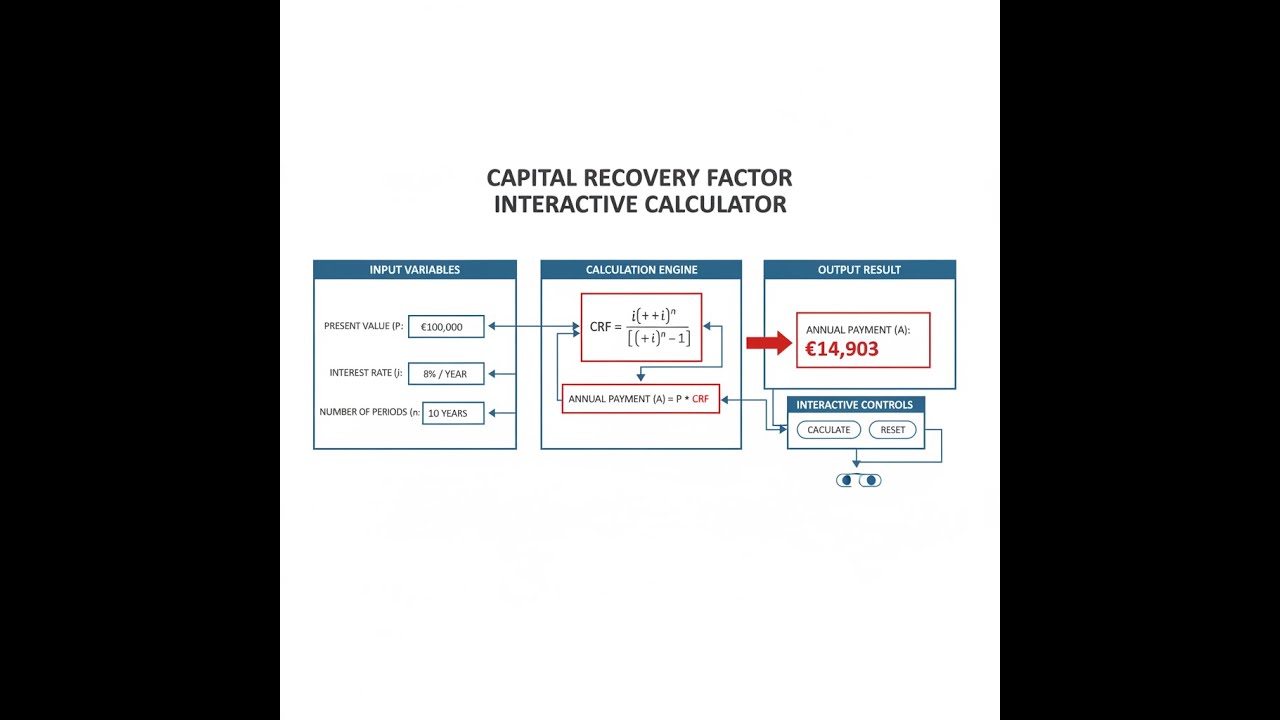
Capital Recovery Factor Interactive Visualizer
Watch how interest rate and project duration affect your required periodic payments to recover capital investments. Adjust parameters to see the CRF formula in action with real-time payment calculations.
CAPITAL RECOVERY FACTOR
0.1490
ANNUAL PAYMENT
$14,903
TOTAL PAYMENTS
$149,029
TOTAL INTEREST
$49,029
FIRGELLI Automations — Interactive Engineering Calculators
Equations & Formulas
Use the formula below to calculate the Capital Recovery Factor.
Capital Recovery Factor (CRF)
CRF = [ i(1 + i)n ] / [ (1 + i)n − 1 ]
where:
CRF = Capital Recovery Factor (dimensionless)
i = interest rate per period (decimal form)
n = number of compounding periods (dimensionless)
Annual Payment (A)
A = P × CRF
where:
A = uniform annual payment ($)
P = present value or initial investment ($)
CRF = Capital Recovery Factor (dimensionless)
Present Value from Payment
P = A / CRF = A × [ (1 + i)n − 1 ] / [ i(1 + i)n ]
This is the present worth factor, the inverse of CRF
Special Case: Zero Interest Rate
CRF = 1 / n (when i = 0)
When no interest is charged, capital is recovered by equal portions over n periods
Simple Example
Initial investment (P): $10,000
Interest rate (i): 10% per year
Number of periods (n): 5 years
CRF = [0.10 × (1.10)5] / [(1.10)5 − 1] = 0.2638
Annual payment (A) = $10,000 × 0.2638 = $2,638 per year
Theory & Engineering Applications
The Capital Recovery Factor represents a fundamental time-value-of-money concept in engineering economics, converting a present lump sum into a series of equivalent uniform periodic payments. Unlike simple amortization that merely distributes principal, CRF accounts for both principal recovery and interest charges, ensuring that lenders or investors receive compensation for the time value of money while recovering the initial capital outlay.
Mathematical Foundation and Derivation
The CRF formula derives from the equivalence between a present sum P and a uniform series of payments A. Starting with the present worth of an annuity formula and solving for the payment term yields the capital recovery relationship. The factor itself is dimensionless, serving as a multiplier that transforms present value into periodic payment requirements. The denominator term [(1 + i)n − 1] represents the accumulated value of one dollar per period at interest rate i, while the numerator i(1 + i)n ensures that both interest and principal are recovered.
A critical but often overlooked aspect is the sensitivity of CRF to interest rate variations. For typical engineering projects spanning 10-30 years, a 1% change in interest rate can alter the recovery factor by 8-15%, dramatically affecting project feasibility. This sensitivity increases with project duration, making long-term infrastructure investments particularly vulnerable to interest rate forecast errors. Engineers must recognize that CRF calculations assume constant interest rates throughout the project life—an assumption that rarely holds in volatile economic environments.
Engineering Economics and Project Evaluation
Capital recovery analysis forms the backbone of replacement studies, lease-versus-buy decisions, and economic service life determination. When evaluating equipment replacement, engineers calculate the equivalent annual cost (EAC) by applying CRF to the initial investment and adding annual operating expenses. The equipment with the lowest EAC over its economic life represents the optimal choice, even if initial costs differ substantially.
In manufacturing environments, CRF enables comparison of automation investments with different lifespans and capital requirements. A $500,000 robotic system with 15-year life competes against a $200,000 conventional system with 8-year life not on initial cost alone, but on equivalent annual cost that incorporates capital recovery, operating expenses, and salvage value considerations. This levelized cost approach prevents bias toward lower initial investments that may prove more expensive over time.
Infrastructure and Public Works Applications
Municipal engineers apply CRF extensively when evaluating water treatment facilities, transportation systems, and power generation projects. These long-duration investments (30-50 years) require careful consideration of discount rates, which represent the minimum acceptable rate of return or opportunity cost of capital. For public projects, the social discount rate—typically 3-7% in developed economies—reflects society's time preference for current versus future benefits.
Rate-setting for public utilities relies fundamentally on capital recovery principles. When a water authority invests $50 million in treatment infrastructure with a 40-year design life, the annual revenue requirement must cover operating costs plus capital recovery sufficient to retire bonds and compensate investors. The CRF calculation determines the portion of user fees allocated to capital costs, ensuring long-term financial sustainability of essential services.
Energy Systems and Life-Cycle Cost Analysis
Renewable energy project economics depend critically on accurate CRF application. Solar photovoltaic installations, wind farms, and battery storage systems involve substantial upfront capital with minimal operating costs spread over 20-30 years. The levelized cost of energy (LCOE)—expressed in dollars per kilowatt-hour—applies CRF to initial investment, then divides by lifetime energy production. This metric enables direct comparison with conventional generation regardless of cost structure differences.
For a commercial solar installation, LCOE calculations reveal how system cost, financing terms, and degradation rates interact. A $2 million system financed at 6% over 25 years yields an annual capital charge of $157,470 (using CRF = 0.078735). When divided by annual production of 3,500,000 kWh with 0.5% annual degradation, the levelized capital cost approaches $0.047/kWh. This granular analysis guides investment decisions and policy incentive structures.
Detailed Worked Example: Manufacturing Equipment Acquisition
Problem: A precision machining company evaluates purchasing a CNC milling center for $385,000. The equipment has an expected service life of 12 years with negligible salvage value. Annual operating and maintenance costs total $42,000 in year one, increasing by $3,200 annually due to wear. The company's minimum attractive rate of return (MARR) is 9.5% annually. Calculate: (a) the capital recovery factor, (b) annual capital recovery payment, (c) total equivalent annual cost in year one, and (d) present worth of total costs over the equipment life.
Solution:
Part (a): Calculate CRF
Given: P = $385,000, i = 0.095, n = 12 years
CRF = [i(1 + i)n] / [(1 + i)n − 1]
CRF = [0.095(1.095)12] / [(1.095)12 − 1]
First calculate (1.095)12 = 2.9716
CRF = [0.095 × 2.9716] / [2.9716 − 1]
CRF = 0.2823 / 1.9716
CRF = 0.14316
Part (b): Annual Capital Recovery Payment
Acapital = P × CRF
Acapital = $385,000 × 0.14316
Acapital = $55,117 per year
Part (c): Equivalent Annual Cost (Year One)
EACyear1 = Acapital + O&Myear1
EACyear1 = $55,117 + $42,000
EACyear1 = $97,117
For the complete analysis including escalating O&M costs, convert the gradient series to equivalent annual cost:
Gradient G = $3,200 per year
Gradient-to-annual factor (A/G, 9.5%, 12) = 4.439
AO&M = $42,000 + $3,200 × 4.439 = $56,205
Total EAC = $55,117 + $56,205 = $111,322 per year
Part (d): Present Worth of Total Costs
Using the present worth factor (inverse of CRF):
PWF = [(1 + i)n − 1] / [i(1 + i)n] = 1 / 0.14316 = 6.9847
PWtotal = EAC × PWF
PWtotal = $111,322 × 6.9847
PWtotal = $777,541
This present worth represents the lump sum today that would be equivalent to all costs over the 12-year period. The analysis shows that while initial investment is $385,000, the true economic burden including operating costs and time value of money approaches $778,000 in present-day dollars.
Limitations and Practical Considerations
CRF analysis assumes constant interest rates and uniform payment intervals—conditions rarely met in practice. Variable rate financing, seasonal cash flows, and inflation introduce complexity requiring more sophisticated present worth models. Additionally, CRF cannot capture non-monetary factors such as technological obsolescence risk, regulatory changes, or strategic value of flexibility.
For projects in developing economies or volatile sectors, the discount rate itself becomes uncertain. Sensitivity analysis across a range of interest rates (typically ±3 percentage points) provides insight into decision robustness. Monte Carlo simulation can model combined uncertainties in interest rates, project life, and salvage values, yielding probability distributions of economic outcomes rather than single-point estimates.
For additional financial engineering tools and calculators, visit the FIRGELLI engineering calculator library.
Practical Applications
Scenario: Fleet Replacement Decision for Logistics Company
Maria, the operations manager for a regional delivery service, needs to decide whether to purchase 15 new delivery vans at $38,500 each or lease them at $725 per month. The vans have an expected service life of 8 years with a salvage value of $6,200. Her company's cost of capital is 7.25% annually. Using the CRF calculator with i=7.25%, n=8, she calculates CRF=0.16384. The annual capital recovery on each van is $38,500 × 0.16384 = $6,308. Adding $2,400 annual operating cost gives EAC of $8,708. The lease option costs $8,700 annually, making purchase marginally favorable when accounting for salvage value. This calculation gives Maria confidence to recommend a $577,500 fleet purchase, knowing the 8-year equivalent annual cost of $130,620 beats leasing by nearly $1,200 per year.
Scenario: Solar Energy Investment Analysis
James, a facility engineer at a pharmaceutical manufacturing plant, proposes installing a 500 kW rooftop solar array costing $1.2 million. The system has a 25-year warranty with expected 0.6% annual degradation. Corporate finance requires 8.5% minimum return on capital investments. Using the calculator with P=$1,200,000, i=8.5%, n=25, James finds CRF=0.09347 and annual capital charge of $112,164. The system produces 750,000 kWh in year one, avoiding $0.11/kWh in utility costs, saving $82,500 annually. After accounting for $8,000 annual maintenance, net annual benefit is $74,500—insufficient to justify the $112,164 capital charge. However, with a 30% federal tax credit reducing net investment to $840,000, the annual capital charge drops to $78,555, making the project economically viable with a positive $4,055 annual cash flow even before considering rising electricity prices.
Scenario: Municipal Water System Expansion
Dr. Patel, the utilities director for a growing city of 85,000 residents, must secure financing for a $12.5 million water treatment plant expansion. The facility will serve the community for 40 years with a municipal bond rate of 4.75% annually. Using the CRF calculator, she determines that CRF=0.05545 for these terms, requiring annual debt service of $693,125. The expansion will serve 18,000 new connections, so each connection must contribute $38.51 annually toward capital costs alone. When Dr. Patel presents this to the city council, she demonstrates that a $3.25 monthly increase in water rates ($39/year) will fully cover the expansion debt service while maintaining the utility's financial sustainability. The CRF calculation provides the transparent, defensible basis for the rate adjustment that the council needs to approve the critical infrastructure investment.
Frequently Asked Questions
Free Engineering Calculators
Explore our complete library of free engineering and physics calculators.
Browse All Calculators →🔗 Explore More Free Engineering Calculators
About the Author
Robbie Dickson — Chief Engineer & Founder, FIRGELLI Automations
Robbie Dickson brings over two decades of engineering expertise to FIRGELLI Automations. With a distinguished career at Rolls-Royce, BMW, and Ford, he has deep expertise in mechanical systems, actuator technology, and precision engineering.
Need to implement these calculations?
Explore the precision-engineered motion control solutions used by top engineers.


