Economic Order Quantity Interactive Calculator

The Economic Order Quantity (EOQ) calculator determines the optimal order quantity that minimizes total inventory costs by balancing ordering costs against holding costs. Manufacturing managers, supply chain professionals, and inventory planners use this fundamental tool to reduce waste, improve cash flow, and maintain efficient stock levels across operations ranging from small warehouses to multinational distribution networks.

📐 Browse all free engineering calculators

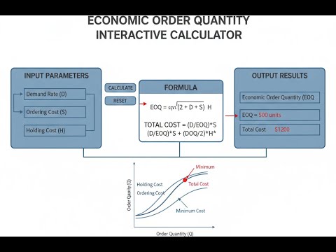
System Diagram

Economic Order Quantity Calculator

Equations & Variables

Variable Definitions

Variable	Description	Units
Q*	Economic Order Quantity (optimal order size)	units
D	Annual demand	units/year
S	Ordering cost (fixed cost per order)	$/order
H	Annual holding cost per unit	$/unit/year
TC	Total annual inventory cost	$/year
ROP	Reorder point (inventory level to trigger new order)	units
d	Daily demand rate (D/365)	units/day
L	Lead time (time from order to delivery)	days
N	Number of orders per year	orders/year
T	Time between orders (cycle time)	days

Theory & Engineering Applications

The Economic Order Quantity model, developed by Ford W. Harris in 1913 and popularized by R.H. Wilson, represents one of the foundational concepts in operations research and supply chain management. This mathematical optimization technique balances two competing cost drivers: the fixed costs associated with placing orders and the variable costs of holding inventory over time. While simple in formulation, the EOQ model reveals profound insights about inventory dynamics that remain relevant across modern manufacturing, distribution, and retail operations.

Fundamental Cost Trade-offs

The genius of the EOQ model lies in its recognition that ordering costs and holding costs move in opposite directions as order quantity changes. When organizations place many small orders, they minimize inventory holding costs—less capital tied up in stock, reduced warehouse space requirements, lower insurance premiums, and decreased obsolescence risk. However, frequent ordering dramatically increases procurement costs through administrative overhead, shipping charges, receiving labor, quality inspection time, and purchase order processing expenses that remain relatively constant regardless of order size.

Conversely, placing large infrequent orders reduces the per-unit ordering cost by amortizing fixed expenses across more units. A company ordering 10,000 units once per year pays the ordering cost once, while ordering 100 units 100 times per year multiplies that fixed cost by 100. Yet large orders create substantial holding costs through warehouse space utilization, inventory insurance at 1-3% of inventory value annually, capital opportunity costs typically calculated at the company's weighted average cost of capital (8-15% for most manufacturers), physical deterioration, technological obsolescence, and shrinkage from theft or damage.

The EOQ formula identifies the precise order quantity where these opposing cost curves intersect, minimizing total inventory cost. Mathematically, this occurs where ordering cost per year equals holding cost per year: (D/Q*)S = (Q*/2)H. This equilibrium condition, derived through calculus by setting the derivative of total cost to zero, produces the square root relationship that defines optimal order quantity.

Holding Cost Components and Practical Estimation

Accurately estimating holding costs proves more challenging than most inventory management textbooks acknowledge. The annual holding cost H encompasses multiple components, each requiring separate quantification. Capital cost represents the largest component for most organizations—the return the company could earn by investing cash elsewhere rather than holding inventory. For a manufacturer with a 12% weighted average cost of capital and a $75 unit cost item, capital cost alone contributes $9.00 per unit per year to holding costs.

Warehouse space costs depend heavily on facility type and geographic location, ranging from $4-8 per square foot annually for basic distribution space in secondary markets to $15-25 per square foot in major metropolitan logistics hubs. A pallet occupying 48 square feet in a $10/sq ft warehouse incurs $480 annual space cost. If that pallet holds 50 units, space cost adds $9.60 per unit per year. Insurance typically ranges from 1-3% of inventory value annually, while obsolescence risk varies dramatically by industry—perhaps 2-5% for stable products like fasteners or pipes, but 15-30% for electronics or fashion items with rapid product lifecycles.

Temperature-controlled storage adds substantial costs. Refrigerated warehouse space costs $20-35 per square foot annually, while frozen storage reaches $35-50 per square foot. Pharmaceutical products requiring validated cold chain management can incur holding costs exceeding 40% of product value annually. These environmental requirements fundamentally alter EOQ calculations, often driving companies toward smaller, more frequent orders despite higher per-order costs.

Ordering Cost Decomposition and Hidden Expenses

While holding costs prove difficult to estimate, ordering costs contain equally subtle components often overlooked in simplified analyses. Purchase order processing costs include requisition preparation, supplier selection and price negotiation, purchase order creation and approval routing, order transmission, acknowledgment verification, and documentation filing. A comprehensive Aberdeen Group study found average purchase order processing costs ranging from $53 for companies with automated e-procurement systems to $506 for organizations relying on manual paper-based processes.

Receiving costs add further expense through dock scheduling, unloading labor, pallet movement to staging areas, quantity verification counting, quality inspection sampling, inventory system updates, and discrepancy resolution when shipments don't match orders. Complex products requiring detailed inspection protocols or hazardous materials demanding special handling procedures can multiply receiving costs by factors of 3-5 compared to standard commodities.

Transportation costs per order vary with shipping method, order size, and distance. LTL (less than truckload) shipments cost $0.50-2.00 per mile depending on freight class and weight, while dedicated truckload shipping provides economies of scale at $1.50-2.50 per mile for loads exceeding 10,000-15,000 pounds. Small parcel shipping through carriers like UPS or FedEx follows complex dimensional weight algorithms and zone-based pricing that can make frequent small shipments prohibitively expensive for dense, heavy items.

Worked Example: Industrial Bearing Manufacturer

Consider Precision Components Inc., a mid-sized bearing manufacturer in Cleveland, Ohio, managing inventory for their most popular product: a sealed ball bearing used in automotive transmissions. The engineering team must determine optimal ordering quantities for the steel balls that form the bearing's rolling elements, purchased from a specialty supplier in Pennsylvania.

Given parameters:

• Annual demand: D = 847,500 steel balls (based on production schedule of 94,167 bearing units, each requiring 9 balls)
• Unit cost: C = $0.73 per steel ball (negotiated contract price)
• Ordering cost: S = $187 per purchase order (including $62 administrative cost, $48 receiving labor, $37 quality inspection, $40 transportation)
• Capital cost: 11.5% of inventory value (company WACC)
• Warehouse space: $7.20 per square foot annually, with steel balls occupying 0.032 square feet per 1,000 units
• Insurance and taxes: 2.1% of inventory value annually
• Obsolescence/damage: 1.3% of inventory value annually (steel balls are stable but subject to rust if improperly stored)

Step 1: Calculate total annual holding cost per unit

Capital cost contribution: $0.73 × 0.115 = $0.08395 per unit per year

Storage cost contribution: $7.20 per sq ft × 0.000032 sq ft per unit = $0.0002304 per unit per year

Insurance and taxes: $0.73 × 0.021 = $0.01533 per unit per year

Obsolescence and damage: $0.73 × 0.013 = $0.00949 per unit per year

Total holding cost: H = $0.08395 + $0.00023 + $0.01533 + $0.00949 = $0.1090 per unit per year (14.9% of unit cost)

Step 2: Calculate Economic Order Quantity

Q* = √[(2 × 847,500 × $187) / $0.1090]

Q* = √[316,725,000 / 0.1090]

Q* = √2,905,045,872

Q* = 53,898 steel balls per order

Step 3: Calculate derived metrics

Number of orders per year: N = 847,500 / 53,898 = 15.72 orders/year

Time between orders: T = 365 / 15.72 = 23.2 days

Average inventory level: Q*/2 = 53,898 / 2 = 26,949 units

Annual ordering cost: (847,500 / 53,898) × $187 = $2,939

Annual holding cost: (53,898 / 2) × $0.1090 = $2,938

Total annual inventory cost: TC = $2,939 + $2,938 = $5,877

Step 4: Calculate reorder point (assuming 12-day lead time)

Daily demand: d = 847,500 / 365 = 2,322 units/day

Reorder point: ROP = 2,322 × 12 = 27,864 units

Analysis and practical implications:

The EOQ calculation reveals that Precision Components should place orders for approximately 53,900 steel balls every 23 days. Notice that at the optimal order quantity, annual ordering costs ($2,939) essentially equal annual holding costs ($2,938)���this balance is the defining characteristic of the EOQ solution and validates the calculation.

The reorder point of 27,864 units slightly exceeds the average inventory level of 26,949 units, indicating that new orders will arrive before inventory depletes to the average level. This makes sense given the 12-day lead time relative to the 23-day order cycle—inventory will fluctuate between approximately 80,800 units (immediately after receiving a new order: 26,900 remaining + 53,900 new) and 26,900 units (just before the next order arrives).

From a cash flow perspective, the average inventory investment equals 26,949 units × $0.73 = $19,673. This capital commitment must be weighed against the inventory cost savings. If Precision Components instead ordered monthly (12 times per year), order quantity would increase to 70,625 units, raising holding costs to $3,849 while reducing ordering costs to $2,244, for a total cost of $6,093—$216 higher annually than the EOQ approach.

Model Limitations and Extensions

The basic EOQ model operates under several assumptions that rarely hold perfectly in practice, creating opportunities for model refinement. The assumption of constant, predictable demand ignores seasonal fluctuations, trend growth, and demand uncertainty. Automotive bearing demand, for instance, follows automotive production cycles with summer peaks and winter troughs. Safety stock calculations and time-series forecasting methods address this limitation by adding buffer inventory proportional to demand variability and lead time uncertainty.

The model assumes instantaneous replenishment—the entire order quantity arrives simultaneously. For manufacturers producing items internally rather than purchasing them, the Economic Production Quantity (EPQ) model modifies the EOQ formula to account for gradual inventory accumulation during production runs. The EPQ formula becomes Q* = √[(2DS) / (H(1 - d/p))] where d represents daily demand rate and p represents daily production rate.

Quantity discounts violate the constant unit price assumption. When suppliers offer price breaks at specific order quantities, total cost must include purchase price: TC = (D/Q)S + (Q/2)H + DC. The optimal order quantity may shift to a discount breakpoint even if it exceeds the calculated EOQ, provided the purchase price savings offset increased holding costs. Evaluating quantity discounts requires calculating total cost at each breakpoint and comparing against the EOQ solution.

Storage capacity constraints may prevent ordering the full EOQ quantity. A warehouse with limited refrigerated space or a retail store with fixed shelf space must respect these physical limits. Constrained optimization techniques using Lagrange multipliers determine the optimal order quantity subject to storage constraints, typically resulting in more frequent orders than the unconstrained EOQ would suggest.

Multiple product interactions create additional complexity. Products competing for the same limited warehouse space or requiring coordinated ordering from a single supplier benefit from joint replenishment models that determine optimal order quantities and ordering intervals across product portfolios. These extensions minimize system-wide costs rather than optimizing individual items in isolation.

Integration with Modern Supply Chain Systems

Contemporary supply chain management increasingly integrates EOQ principles within larger optimization frameworks. Enterprise Resource Planning (ERP) systems like SAP and Oracle embed EOQ calculations within material requirements planning (MRP) modules, automatically adjusting order quantities based on current cost parameters, demand forecasts, and supplier lead times. Advanced planning systems extend basic EOQ logic with constraint-based optimization considering production capacity, transportation economies, and inventory budget limitations simultaneously.

Vendor-managed inventory (VMI) arrangements shift ordering responsibility to suppliers who monitor customer inventory levels and automatically replenish stock according to agreed parameters. VMI systems often use modified EOQ models where the supplier optimizes total supply chain costs rather than individual party costs, potentially benefiting both parties through reduced bullwhip effect and better demand visibility. A bearing supplier implementing VMI for Precision Components might adjust delivery frequency based on their production schedule efficiency rather than pure EOQ optimization.

Just-in-time (JIT) and lean manufacturing philosophies challenge the fundamental EOQ premise that holding inventory provides value. JIT practitioners argue that inventory hides problems—quality defects, machine unreliability, supplier inconsistency—and that organizations should attack root causes rather than buffer against them with inventory. In practice, successful JIT implementations reduce both setup times (lowering S) and lead times (reducing safety stock requirements), which naturally drives EOQ calculations toward smaller, more frequent orders without abandoning the underlying cost minimization logic.

For more insights into optimizing manufacturing and industrial systems, explore additional resources in the engineering calculator library.

Practical Applications

Frequently Asked Questions