If either the sound source or the observer is moving, the frequency you hear isn’t what’s actually being emitted. Calculating that difference is what matters in engineering. This Doppler Effect Calculator handles the numbers for you—whether you’re finding observed frequency, source velocity, observer velocity, wave speed, or relative velocity based on source frequency, wave speed, and the motions involved. It comes up everywhere from radar to medical ultrasound to astronomy, wherever a shift in wave frequency has to be quantified. Below you’ll find the main equation, a full step-by-step example for aircraft radar, some background on why the effect happens, and a FAQ.
What is the Doppler Effect?
The Doppler Effect is a frequency change that happens when there’s motion between the wave source and the observer. Coming closer means the pitch goes up. Moving apart, it drops.
Simple Explanation
Picture a spinning sprinkler: you get sprayed more often as it points toward you, less often when it’s swinging away. Sound acts the same way. When something emitting sound moves toward you, the waves get packed closer together (higher pitch); move away, and the waves stretch out (lower pitch). That’s the Doppler Effect—you’re hearing how motion changes the arrival rate of wavefronts.
📐 Browse all 1000+ Interactive Calculators
How to Use This Calculator
- Choose what you need to solve for from the dropdown—could be observed frequency, source velocity, observer velocity, wave speed, or relative velocity.
- Fill in any known values shown: source frequency (Hz), wave speed (m/s), source velocity (m/s), and/or observer velocity (m/s)—whatever makes sense for the calculation you’re running.
- If your chosen mode needs it, you’ll see an input for observed frequency (f') in Hz.
- Hit Calculate. The result will show up below.
Doppler Effect Diagram

Interactive Doppler Effect Calculator
This calculator is intended for education, concept evaluation, and preliminary design. Results are based on the equations and assumptions described on this page, but cannot account for every real-world load case, tolerance, material property, environmental condition, installation detail, safety factor, code, or regulatory requirement. Verify all inputs, assumptions, units, and results independently before selecting components or using the result in a real application. Safety-critical, structural, medical, lifting, transportation, or regulated applications must be reviewed by a qualified engineer.
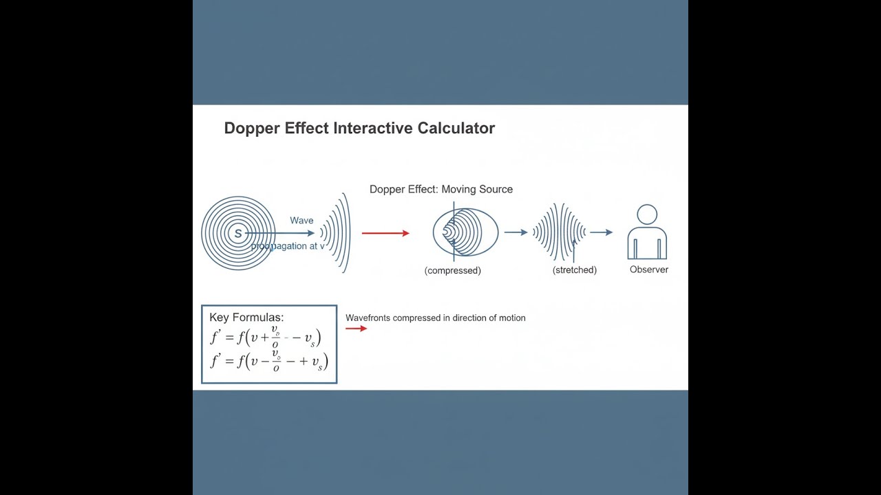
Doppler Effect Interactive Visualizer
Move the sliders to adjust source and observer velocities and see in real time how the frequency you get out changes. The animation gives a direct look at how the wavefronts squeeze or spread, not just as a diagram but with numbers tied to your inputs.
OBSERVED FREQ
467 Hz
FREQ SHIFT
+27 Hz
PERCENT CHANGE
+6.1%
FIRGELLI Automations — Interactive Engineering Calculators
Governing Equations
This is the equation you’ll use to work out observed frequency from the knowns (source frequency, wave speed, and velocities):
General Doppler Effect Formula
f' = f₀ × [(v + vo) / (v - vs)]
Where:
- f' = observed frequency (Hz)
- f₀ = source frequency (Hz)
- v = wave propagation speed in medium (m/s)
- vo = observer velocity (m/s, positive toward source)
- vs = source velocity (m/s, positive toward observer)
Frequency Shift
Δf = f' - f₀
Where:
- Δf = frequency shift (Hz)
- Positive Δf indicates higher observed frequency (blueshift)
- Negative Δf indicates lower observed frequency (redshift)
Observed Wavelength
λ' = v / f'
Where:
- λ' = observed wavelength (m)
- Wavelength inversely proportional to observed frequency
- Compressed wavelengths for approaching sources
Relativistic Doppler Effect (Electromagnetic Waves)
f' = f₀ × √[(1 - β) / (1 + β)]
Where:
- β = vrel / c (velocity ratio)
- vrel = relative velocity (m/s, positive for recession)
- c = speed of light (2.998 × 10⁸ m/s)
- Required for velocities above ~10% of wave speed
Simple Example
A 440 Hz source (with observer not moving, v_o = 0) heads toward you at 20 m/s. Speed of sound is 343 m/s.
Plug into the formula: f' = 440 × (343 + 0) / (343 − 20) = 440 × 343 / 323 = 467.2 Hz
This is a +27.2 Hz shift, which is about half a musical semitone—noticeable by ear.
Theory & Practical Applications
The Doppler Effect shows up whenever there’s relative motion between a wave source and an observer—the received frequency won’t match the emitted one. This is a direct result of the way the moving source or observer changes how often wavefronts arrive. It isn’t limited to sound; you see it anywhere waves travel and something moves, though the specifics change for things like light at high speed. The typical Doppler formula here works for sound and other waves in a medium. For electromagnetic waves (like light or radar), you need a slightly different approach if you’re dealing with speeds near that of light.
Physical Mechanism and Wave Compression
If a source is heading toward the observer, each wavefront gets launched from a spot closer than the last, so the crests bunch up. For a source at velocity vs toward you, the wavelength shrinks by (v - vs)/v. That shrinkage bumps up the observed frequency: f' = v/λ'. The closer together those crests, the higher the pitch (or bluer the light).
The Doppler effect isn’t perfectly symmetric: moving the source and moving the observer produce different results for the same velocity, as long as there’s a medium like air or water involved. Source motion squeezes wavefronts closer or farther apart in the medium; observer motion just makes you intercept crests at a different rate. For light or other electromagnetic waves in vacuum, only the relative velocity matters, and you use the relativistic formula.
Radar and Velocity Measurement Systems
Traffic radar typically uses 24.15 GHz or 34.7 GHz, sending out a steady wave that bounces off vehicles. The frequency shift in the reflected signal comes from two effects: once when it hits a moving vehicle and again when it bounces back—so it’s a double Doppler shift. The math says Δf = 2f₀v/c (c = speed of light). For a 30 m/s car and 24.15 GHz radar, the shift is about 4.83 kHz—plenty for electronics to pick up.
Because the shift doubles, so do any errors in measuring the actual speed or the exact radar angle. If the radar isn’t pointed straight ahead, the number you get is always a bit low—at a 20° angle, the reading is about 6% less than the true speed. Lidar sidesteps the Doppler effect by measuring time-of-flight, using short light pulses instead.
Medical Ultrasound Doppler Imaging
In ultrasound, Doppler measures how fast blood is moving by tracking frequency shifts in reflected sound. These systems usually work at 2–10 MHz. Blood cells moving toward the probe reflect higher frequencies, away means lower. The shift depends on both the actual velocity and the angle between the probe and the flow: Δf = 2f₀v·cos(θ)/c, with c ~1540 m/s in tissue. The cosine term means things get tricky if your angle gets too steep—at 80°, you lose 83% of your signal compared to a beam more in line with the vessel. That limits where you can position the probe. Color Doppler assigns these frequency shifts to color, highlighting details like turbulent flow in vessels. Pulse Doppler lets you pick out flow at a specific depth, but with a tradeoff in time resolution.
Astronomical Spectroscopy and Redshift
In astronomy, the Doppler shift shows up as spectral lines moving due to motion—like the sodium D-line shifting as stars or galaxies move toward or away from us. The speed calculation is straightforward for slow speeds, but at a big fraction of light speed, use the relativistic equation. Measuring tiny shifts in star spectra even lets us spot planets tugging on stars. For example, a 12.5 m/s wobble creates a shift requiring spectrometers with extremely high precision—down to one part in hundreds of millions.
Worked Example: Aircraft Doppler Radar Navigation
Problem: An aircraft moving at 215 m/s sends a 13.325 GHz radar beam 45° ahead and measures the reflected signal from the ground. Find: (a) what’s the Doppler shift from the motion, (b) the double shift from transmit and return, (c) how much error shows up if turbulence changes the angle by 2°, and (d) what are the wavelengths involved?
Given values:
- Aircraft velocity: v = 215 m/s
- Transmitted frequency: f₀ = 13.325 GHz = 1.3325 × 10¹⁰ Hz
- Beam angle to ground: θ = 45°
- Speed of light: c = 2.998 × 10⁸ m/s
- Perturbed angle: θ' = 47°
Solution:
(a) Single Doppler shift frequency:
First, project aircraft speed along the radar beam: v·cos(45°). The shift (for these slow speeds) is:
Δf₁ = f₀ × (v·cos(θ)/c)
Δf₁ = 1.3325×10¹⁰ × (215 × cos(45°) / 2.998×10⁸)
Δf₁ = 1.3325×10¹⁰ × (152.03 / 2.998×10⁸)
Δf₁ = 1.3325×10¹⁰ × 5.072×10⁻⁷
Δf₁ = 6,758 Hz = 6.758 kHz
(b) Double-Doppler shift observed by radar:
Because the ground reflects back (effectively a second moving target), double the shift:
Δftotal = 2 × Δf₁
Δftotal = 13,516 Hz = 13.516 kHz
The new frequency is 13.325000000 GHz + 0.000013516 GHz = 13.325013516 GHz. The fractional shift is tiny, but radar hardware can measure this with no trouble.
(c) Velocity error from 2° angle drift:
Now use a 47° beam angle in the formula:
Δf'total = 2f₀ × (v·cos(47°)/c)
Δf'total = 2 × 1.3325×10¹⁰ × (215 × 0.6820 / 2.998×10⁸)
Δf'total = 13,022 Hz
To see what the radar thinks the speed is:
vmeasured = (Δf'total × c) / (2f₀ × cos(45°))
vmeasured = (13,022 × 2.998×10⁸) / (2 × 1.3325×10¹⁰ × 0.7071)
vmeasured = 206.9 m/s
This is 8.1 m/s off; a 3.8% error just from a 2° angle shift.
Doppler navigation can’t ignore small angle errors. Typical systems compensate with additional sensors that keep the beam locked, or correct the math in real time for drift.
(d) Transmitted and received wavelengths:
λtransmitted = c / f₀ = 2.998×10⁸ / 1.3325×10¹⁰
λtransmitted = 0.0225 m = 22.5 mm (K-band)
λreceived = c / f' = 2.998×10° / 1.3325013516×10¹⁰
λreceived = 0.022499977 m = 22.499977 mm
The 23-nanometer change seems minor, but radar phase detectors can work with even smaller differences, extracting velocity by comparing many cycles over time.
Practical Limitations and Edge Cases
The main Doppler formula stops working if the velocity approaches wave speed. With sound in air at 343 m/s, a 300 m/s source heading straight toward you gives a much bigger frequency jump—over 7×. If the source hits the speed of sound, theoretically the frequency "goes infinite," but in real life, that’s where you get shock waves (not just higher pitch), and you need different analysis for those cases.
If an object moves across your field of view (perpendicular motion), classical Doppler shift vanishes, but relativity says you still get a tiny shift from time dilation, on the order of (v/c)². For things like satellites or GPS, this is measurable and has to be corrected, but for most uses, it’s negligible. GPS in particular has to correct for both this velocity effect and for gravitational redshift to achieve precise timing.
Optical or laser Doppler systems (like for wind speed) have to factor in atmospheric refraction, which bends the beam and changes the actual angle. This can cause small but relevant errors for precision work—for typical environmental measurements, it’s usually negligible, but you can't ignore it in boundary-layer wind profiling. Corrections are made based on atmospheric models or by combining readings from several angles.
Frequently Asked Questions
▼ Why does the Doppler formula treat source and observer motion differently?
▼ How does temperature affect Doppler radar measurements?
▼ Can Doppler shift be used to measure absolute distance or only velocity?
▼ What causes the siren pitch to change abruptly as an ambulance passes, not gradually?
▼ Why do police radar detectors warn before the radar unit can measure vehicle speed?
▼ How does cosmological redshift differ from Doppler redshift?
Free Engineering Calculators
Explore our complete library of free engineering and physics calculators.
Browse All Calculators →🔗 Explore More Free Engineering Calculators
About the Author
Robbie Dickson — Chief Engineer & Founder, FIRGELLI Automations
Robbie Dickson brings over two decades of engineering expertise to FIRGELLI Automations. With a distinguished career at Rolls-Royce, BMW, and Ford, he has deep expertise in mechanical systems, actuator technology, and precision engineering.
Need to implement these calculations?
Explore the precision-engineered motion control solutions used by top engineers.


