Optical Fiber Attenuation Interactive Calculator

When you're laying out a fiber optic link, you need to figure out every single decibel of loss—fiber, connectors, splices—before thinking about whether your transceivers and amplifiers will cut it, or if your planned run is too long. This Optical Fiber Attenuation Calculator lets you plug in the numbers for fiber length, attenuation rate, how many connectors there are, and splices to see how much signal you'll lose overall. It's a step you can't skip for any telecom system, data center links, or subsea cables—if you get the math wrong, the link might not work. Scroll down for the main calculation, a real-world example, detailed engineering notes, and quick answers to frequent questions.

What is optical fiber attenuation?

Optical fiber attenuation is just how much optical signal you lose as it travels through the fiber. It's measured in decibels (dB). You need to know how many dB you'll lose over the length of fiber and through each connector or splice along the route.

Simple Explanation

It's a bit like water pressure dropping the longer and more complicated your hose gets. In fiber, every kilometer, connector, and splice chips away at your signal level. Add them up—that’s your total loss to plan for.

📐 Browse all 1000+ Interactive Calculators

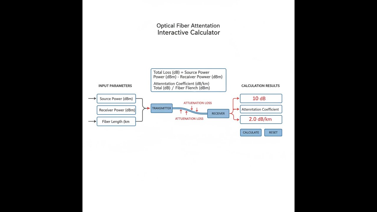
Fiber Attenuation Diagram

Optical Fiber Attenuation Calculator

How to Use This Calculator

1. Pick the calculation mode—total loss, output power, max length, etc.
2. Enter your fiber length (km), the fiber’s attenuation rate (dB/km), how many connectors and splices you're using, and their loss values.
3. If your calculation needs it, add in input or output power values.
4. Hit Calculate to see the answer.

Attenuation Equations

Here’s the equation for total attenuation in a fiber run.

Here’s the formula for output power after losses in your link.

Here's how you solve for the maximum fiber length before you run out of power budget.

Link margin tells you how much signal headroom you have at the receiver.

Simple Example

Say your fiber is 10 km long, the attenuation coefficient is 0.35 dB/km, you have 2 connectors at 0.5 dB each, 3 splices at 0.1 dB each, and your input power is 0 dBm.

Fiber loss: 0.35 × 10 = 3.5 dB. Connector loss: 2 × 0.5 = 1.0 dB. Splice loss: 3 × 0.1 = 0.3 dB.

Total attenuation: 3.5 + 1.0 + 0.3 = 4.8 dB. Output power: 0 − 4.8 = −4.8 dBm.

Theory & Engineering Applications

Fiber attenuation is the main thing that limits how far and reliably you can send optical signals. Once you know the loss, you can plan how long a run you can use before you need an amplifier or regeneration, or whether your chosen transceivers will work for that distance. This matters in telecom, data centers, underwater links, and sensor networks—a proper estimate keeps you from running into signal shortfalls or overspending on unnecessary upgrades.

Physical Mechanisms of Fiber Attenuation

Signal loss in fiber comes down to two main causes: absorption and scattering. Absorption happens when light gets absorbed by the glass itself, either from the material’s atomic bonds (intrinsic) or from impurities (extrinsic) like OH⁻ ions left over from manufacturing, with a strong effect near 1383 nm. Modern fiber is pretty clean—"low water peak" fiber is standard—so this is mostly under control if you buy decent product.

Rayleigh scattering—invisible, tiny variations in the glass—limits how good fiber can get. It’s much worse at shorter wavelengths because scattering scales with λ⁻⁴ (wavelength to the -4). That’s why single-mode fiber at 1550 nm is far lower loss than multimode fiber at 850 nm. For real numbers, expect 2.5 dB/km at 850 nm (multimode), 0.35 dB/km at 1310 nm, and down to 0.20 dB/km or better at 1550 nm for typical single-mode fiber if the manufacturer’s specs check out.

Connector and Splice Losses

Aside from the fiber itself, you also get loss at every connector and splice. Connectors lose signal mostly through misalignment, dirt, imperfect end-faces, and tiny air gaps. Basic PC-type connectors are about 0.3–0.5 dB loss on a good day; APC (angled type) connectors reduce back-reflection at the expense of sometimes a bit more insertion loss (maybe 0.5–0.8 dB). If you keep connectors clean and mated properly, you stay near the low end of that range.

Splices are better—but only if done right. Fusion splices (real arc-welds) are usually under 0.1 dB each; mechanical splices are more variable, from 0.1 up to 0.3 dB. In a long route with lots of patch panels and repair joints, splice and connector loss can actually beat fiber loss itself, so keep joint count as low as you can, and spec good installers.

Wavelength-Dependent Attenuation and Spectral Windows

Telecom gear sticks to certain wavelength windows for good reason: 1310 nm (O-band) has zero chromatic dispersion in standard single-mode fiber but a bit more loss, while 1550 nm (C-band) has minimum loss and supports standard EDFAs (fiber amplifiers), making it the main choice for long-distance systems. L-band (above 1565 nm) gets used if you really need the bandwidth and can handle the slight penalty in loss.

Temperature changes matter, but are easy to overlook. As temperature rises, fiber loss goes up by about 0.001 dB/km per °C above 20°C, which can add up over tens of kilometers or in harsh locations. For critical long runs, plan a margin for the environment—don’t trust a single lab measurement at room temperature.

Worked Example: Data Center Interconnect Link Budget

Suppose you need to run a 15.7 km fiber link at 1310 nm between two data centers. The transceivers put out +2 dBm, you know the minimum receiver spec is -18 dBm, and you want a 3 dB margin. There will be 6 connectors (let’s assume 0.4 dB loss each) and 2 fusion splices (0.08 dB each).

Step 1: Available Power Budget

Budget = Output power - Receiver sensitivity - Margin = (+2) - (–18) – (3) = 17 dB

Step 2: Connector Loss

6 × 0.4 = 2.4 dB

Step 3: Splice Loss

2 × 0.08 = 0.16 dB

Step 4: Budget Left for Fiber

17 – 2.4 – 0.16 = 14.44 dB

Step 5: Max Allowable Fiber Loss

14.44 dB over 15.7 km is 0.92 dB/km. That’s much higher than typical fiber, so the link is fine. If your actual fiber is 0.35 dB/km, real fiber loss is 15.7 × 0.35 = 5.50 dB.

Step 6: Check Total Loss and Margin

All-in link loss: 5.50 + 2.4 + 0.16 = 8.06 dB. Received power: +2 – 8.06 = –6.06 dBm. That’s 11.94 dB above the receiver sensitivity spec, so you have margin for aging, future repairs, fiber stress, and climate shifts. If that's too much margin, you might downgrade to a cheaper transceiver or stretch for a longer link.

Nonlinear Effects and High-Power Limitations

For most fiber runs, linear loss is all you need to worry about. But at higher launch powers (usually above +6 or +10 dBm), fiber starts exhibiting non-linear effects: Stimulated Raman Scattering transfers energy between channels, while Stimulated Brillouin Scattering sends some light backwards, capping how much power gets through on a single channel. For dense WDM systems, Four-Wave Mixing can inject unwanted signals into neighboring channels, especially at high power density or low channel spacing. These effects mean that past a certain power, extra input doesn't help—your limiting factor changes from receiver sensitivity to whatever the fiber itself can tolerate.

Amplifier Spacing and Regeneration Requirements

Long-haul links (hundreds or thousands of km) use optical amplifiers (EDFAs, usually) to boost the signal periodically. The real-world spacing between amplifiers depends on fiber loss and how much loss-per-span your amplifiers can handle. With 0.20 dB/km loss at 1550 nm and a typical 20–30 dB amplifier gain, you get 80–100 km per hop before OSNR (noise ratio) becomes the issue. Subsea cable designs push this with specialty fiber (0.16 dB/km or so) and carefully spaced repeaters. But no matter what, you eventually hit the wall with accumulated amplifier noise and fundamental fiber loss. That’s what sets the true long-distance records—and drives up the cost per kilometer.

For more engineering calculators, check out the engineering calculator library.

Practical Applications

Frequently Asked Questions

Video Walkthrough - How to Use This Calculator