Building a long-distance signal link is mostly about reducing the amount of signal you lose over that distance. Every meter adds some loss (attenuation). If you don’t account for it and your signal falls below the noise floor, the receiver can’t make sense of it. The Attenuation Calculator lets you figure out signal power loss, remaining output power, the attenuation coefficient, max distance for a given loss, or the direct power ratio. Getting link budgets right is basic practice in fiber optics, RF lines, and underwater acoustic links—get it wrong and you’re troubleshooting dead links instead of finishing an install. This page shows key formulas, a practical fiber optic example, straightforward explanations of attenuation mechanisms, and answers to real engineering questions.
What is signal attenuation?
Signal attenuation means loss of power as a signal moves through something—could be cable, fiber, water, or air. The farther the signal travels, the weaker it becomes.
Simple Explanation
It’s like water pressure dropping in a long hose: friction inside the hose slowly eats away at the pressure. For signals, energy leaks out into the material around it (by absorption or scattering), so your output is always less than your input. The attenuation coefficient quantifies how quickly that loss stacks up over distance.
📐 Browse all 1000+ Interactive Calculators
Visual Diagram: Signal Attenuation Through Medium

How to Use This Calculator
- Pick what you want to solve: total attenuation, output power, attenuation coefficient, distance, power ratio, or dB/linear conversions.
- Put in your input power and unit (dBm, Watts, or mW). Fill in the other required values like attenuation coefficient and distance, and make sure you select the right units for what you’ve measured.
- Make your units line up (distance and attenuation coefficient) — the calculator converts units for you if you select them correctly.
- Click Calculate.
Attenuation Interactive Calculator
This calculator is intended for education, concept evaluation, and preliminary design. Results are based on the equations and assumptions described on this page, but cannot account for every real-world load case, tolerance, material property, environmental condition, installation detail, safety factor, code, or regulatory requirement. Verify all inputs, assumptions, units, and results independently before selecting components or using the result in a real application. Safety-critical, structural, medical, lifting, transportation, or regulated applications must be reviewed by a qualified engineer.
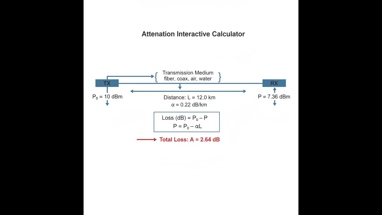
Signal Attenuation Interactive Visualizer
You can watch signal power drop exponentially as it moves through different media. Adjust input power and attenuation coefficients to get real-time output power, total loss, and linear ratio calculations.
OUTPUT POWER
6.0 dBm
TOTAL LOSS
4.0 dB
POWER RATIO
0.398
LINEAR POWER
3.98 mW
FIRGELLI Automations — Interactive Engineering Calculators
Attenuation Equations
Use the formula below to calculate total signal attenuation.
Total Attenuation (dB):
A = α × L
Where:
- A = Total attenuation (dB)
- α = Attenuation coefficient (dB/km or dB/m)
- L = Distance or path length (km or m)
Use the formula below to calculate output power on the dB scale.
Output Power (dB scale):
P = P₀ - A = P₀ - α × L
Where:
- P = Output power (dBm or dBW)
- P₀ = Input power (dBm or dBW)
Use the formula below to calculate the linear power ratio.
Power Ratio (Linear scale):
P/P₀ = 10(-A/10) = e(-αL)
Where:
- P/P₀ = Linear power ratio (dimensionless)
- α = Attenuation coefficient in Nepers/m when using exponential form
Use the formula below to convert between dB and linear power ratio.
dB to Linear Conversion:
AdB = 10 × log₁₀(P₀/P) = -10 × log₁₀(P/P₀)
Use the formula below to convert between Nepers and decibels.
Neper to dB Conversion:
AdB = 8.686 × ANp
Where:
- ANp = Attenuation in Nepers
- 8.686 = Conversion factor (20/ln(10))
Simple Example
A fiber optic signal enters a 10 km cable with an attenuation coefficient of 0.2 dB/km at an input power of 0 dBm (1 mW).
- Total attenuation: A = 0.2 × 10 = 2.0 dB
- Output power: P = 0 dBm − 2.0 dB = −2.0 dBm
- Linear power ratio: 10^(−2.0/10) = 0.631 — meaning 63.1% of the original power reaches the far end.
Theory & Practical Applications of Signal Attenuation
When a signal travels down a cable, through the air, fiber, or even underwater, it loses strength because the medium saps energy through different mechanisms. This isn’t the same as free space loss, which is mostly about how a signal spreads out. For cables and fibers, signal strength falls off exponentially as it goes, dictated by a few key physical effects—absorption, scattering, and conversion of your signal’s energy to heat. Understanding these lets you size your link, decide where you might need repeaters or amplifiers, and pick technology that’s actually suitable for the job.
Physical Mechanisms of Attenuation
The attenuation coefficient α tells you how quickly signal loss adds up per meter or kilometer. In optical fiber, ‘Rayleigh scattering’ is the main cause near 1550 nm: tiny imperfections in the glass matrix knock photons out of line, and this gets worse at shorter wavelengths due to the λ⁻⁴ dependence. That’s why IR wavelengths perform better than visible light in silica fiber. Material absorption adds more loss, especially around certain wavelengths—water (OH⁻) peaks at 1383 nm, and the glass itself tacks on loss in the deeper infrared.
In coaxial cable and waveguides, two main things rob the signal: resistance in the conductors (made worse at higher frequencies through the ‘skin effect’) and energy lost in the insulation (dielectric loss). As frequency rises, the skin depth shrinks, cramming current into a thinner shell and raising resistance; the relationship goes roughly with the square root of frequency. Dielectric loss, on the other hand, increases more directly with frequency and with the loss tangent of your insulation material.
If you’re sending sound underwater, loss is a mix of energy being absorbed (turned into heat at the molecular level), plus scattering from debris or bubbles. The Thorp equation is a practical way to estimate absorption in seawater, and as frequency rises, absorption climbs very quickly—a few kHz is usable for kilometers, but by 100 kHz even a few hundred meters becomes a stretch.
Link Budget Analysis and System Design
Designing a communication system starts with a link budget—add up all power losses (cables, connectors, mainline medium), subtract them from your transmitter power, and see if you still meet your receiver’s sensitivity spec with some margin. For guided media like fiber and cable, attenuation (α × distance) is the main loss — for RF links, free-space loss dominates. Fiber systems, especially across oceans, are limited by how often you need to boost the signal with amplifiers. Modern low-loss fibers get down to 0.18–0.20 dB/km, but over 6000 km you pile up over 1000 dB of loss. That’s why amplifiers (EDFAs) go in every 40–80 km. Fewer dB per km means fewer amplifiers and lower project costs.
RF coax attenuates much faster as frequency increases. For example, RG-58 is tolerable at 100 MHz but gets brutal at 1 GHz. Upgrading cable to LMR-400 or 7/8” hardline helps but at a price and with tougher installs. Weigh the cost of lower-loss cable against the need for more transmitter power and the risk of unacceptable loss at your highest frequencies.
Worked Example: Fiber Optic Network Design
Problem: Design a metro fiber link (47.3 km) between a headend and a remote cell tower. You have a +3.0 dBm TX at 1550 nm, fiber loss is 0.21 dB/km, required RX sensitivity is -28.0 dBm, and you’ll eat an extra 2.8 dB in connectors/splices. Figure: (a) total attenuation, (b) received power, (c) link margin, (d) if you need amplification, (e) if so, where and what gain for a single EDFA?
Solution:
(a) Total Link Attenuation:
Fiber: 0.21 × 47.3 = 9.933 dB
Connectors/splices: 2.8 dB
Total: 9.933 + 2.8 = 12.733 dB
(b) Received Optical Power:
+3.0 dBm − 12.733 dB = -9.733 dBm
(c) Link Margin:
-9.733 dBm – (–28.0 dBm) = 18.267 dB margin
That’s a healthy excess; you don’t need an amplifier now, and you have slack for fiber aging and repairs down the road.
(d) Amplification Assessment:
No amplifier needed; 3–6 dB margin is standard, you have more than 18 dB.
(e) Hypothetical Amplifier Example:
If you had a 180 km run at the same loss rate, you’d have 40.6 dB loss total. Received power would be +3.0 – 40.6 = -37.6 dBm, which is 9.6 dB too low. Put an amplifier halfway (90 km): you’d see 20.3 dB loss to mid-span, so input at that point is -17.3 dBm. To deliver required power at the far end (plus 3 dB margin), you’d need the amp’s output to be -4.7 dBm (–25.0 + 20.3), so about +12.6 dB gain from that amplifier. This kind of design keeps amplifier noise and distortion low, as you’re using it well below maximum output.
Industry Applications and Standards
There are design tools for link budgets, RF losses, antennas, and modulation in our engineering calculator collection.
Standards like ITU-T G.652 list typical fiber loss limits—for example, ≤0.40 dB/km at 1310 nm and ≤0.30 dB/km at 1550 nm, with real-world cable often doing a bit better. Bend-insensitive fiber per ITU-T G.657 has a slightly higher straight-line loss but won’t dump all your signal at tighter bends; this is worth it in cramped installation routes.
Coax cable specs show loss versus frequency so you can quickly match cable types to your required runs. Long cables in distributed antenna setups eat up RF power fast, sometimes sending most of your transmitter’s output into cable loss unless you switch to fiber-fed remote electronics at the antennas.
Underwater acoustic links are even tougher—absorption rises fast above 10 kHz, so range and data rate trade directly. A 5 km run at 10 kHz faces both absorption and geometric spreading; at higher frequencies, you’ll need relay nodes much closer together to get any signal through at all.
Temperature and Environmental Effects
The loss per meter or km you measure in the lab isn’t always what you get in the field. Fiber attenuation shifts slightly with temperature—about 0.0001 dB/km per °C. Over a 110°C swing, a 50 km link could see about 0.55 dB extra loss, which can matter in marginal or submarine links.
For coax, warm temperatures bump up attenuation via changes in conductor resistance and spacing. LMR-400, for example, rises by about 0.15% per degree above 20°C, so if you have 7.0 dB loss at room temp, it’s 7.53 dB at 70°C. Military and aerospace systems always factor these in for worst-case budgets.
In seawater, temperature, salinity, and pH all affect attenuation. Warm water means higher absorption for acoustics—about 3% more per degree. In the ocean, thermocline layers can make parts of a route even worse or better; these swings can be 10–20 dB up or down from the simple calculation, so robust comms systems need power and coding headroom, not just theoretical loss numbers.
Frequently Asked Questions
Free Engineering Calculators
Explore our complete library of free engineering and physics calculators.
Browse All Calculators →🔗 Explore More Free Engineering Calculators
About the Author
Robbie Dickson — Chief Engineer & Founder, FIRGELLI Automations
Robbie Dickson brings over two decades of engineering expertise to FIRGELLI Automations. With a distinguished career at Rolls-Royce, BMW, and Ford, he has deep expertise in mechanical systems, actuator technology, and precision engineering.
Need to implement these calculations?
Explore the precision-engineered motion control solutions used by top engineers.


