Harmonic Wave Equation Interactive Calculator

The harmonic wave equation calculator enables engineers and physicists to analyze sinusoidal wave propagation across mechanical systems, electromagnetic fields, and acoustic environments. This tool solves for displacement, velocity, acceleration, phase relationships, and energy transport in wave systems where understanding temporal and spatial characteristics is critical for system design, vibration analysis, and signal processing applications.

📐 Browse all free engineering calculators

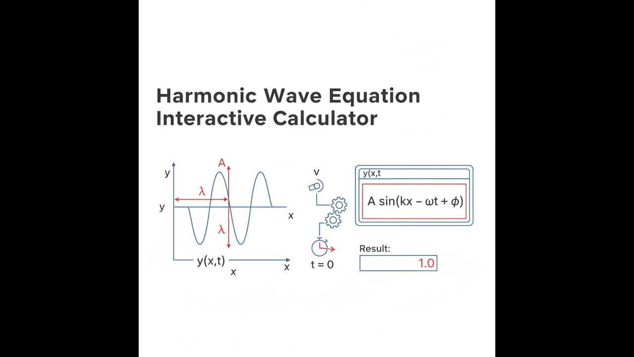
Wave Propagation Diagram

Interactive Harmonic Wave Calculator

Harmonic Wave Equations

Theory & Practical Applications

Physical Foundation of Harmonic Waves

The harmonic wave equation describes sinusoidal disturbances propagating through a medium without net transport of matter. The mathematical form y(x,t) = A sin(kx - ωt + φ) represents a solution to the one-dimensional wave equation ∂²y/∂x² = (1/v²)∂²y/∂²t, which emerges from applying Newton's second law to a continuous elastic medium. The negative sign in the phase argument (kx - ωt) indicates rightward propagation; reversing this sign produces leftward propagation. The wave number k quantifies spatial periodicity while angular frequency ω captures temporal oscillation, with their ratio defining the phase velocity v = ω/k—the speed at which wave crests propagate through the medium.

A critical non-obvious characteristic of harmonic waves is that particle velocity v_particle = ∂y/∂t and wave speed v are fundamentally different quantities. The particle velocity describes local transverse motion of medium elements perpendicular to propagation direction, reaching maximum Aω when displacement crosses equilibrium. Wave speed represents how fast the waveform pattern translates through space and depends exclusively on medium properties—for strings, v = √(T/μ) where T is tension. Engineers frequently encounter confusion when vibration sensors measure particle velocity (proportional to ω) rather than displacement (proportional to A), particularly at high frequencies where velocity dominates even for small displacements. This distinction becomes critical in seismic monitoring where ground particle velocities determine structural loading while wave speeds determine arrival times.

Phase Relationships and Interference

The phase constant φ determines initial displacement and velocity conditions at t = 0, x = 0. For φ = 0, the wave begins at equilibrium with positive velocity. For φ = π/2, it starts at maximum positive displacement with zero velocity. When two harmonic waves with identical frequency and amplitude but different phase constants superimpose, the resulting displacement follows y_total = A₁sin(kx - ωt + φ₁) + A₂sin(kx - ωt + φ₂). Using trigonometric identities, this simplifies to a single harmonic wave with amplitude A_resultant = √(A₁² + A₂² + 2A₁A₂cos(Δφ)), where Δφ = φ₂ - φ₁. Constructive interference occurs when Δφ = 2πn (n integer), yielding A_resultant = A₁ + A₂. Destructive interference at Δφ = π(2n+1) produces A_resultant = |A₁ - A₂|.

Standing wave formation represents a special interference case where waves of equal amplitude travel in opposite directions. The superposition y = Asin(kx - ωt) + Asin(kx + ωt) = 2Asin(kx)cos(ωt) produces nodes (zero displacement at all times) where sin(kx) = 0, occurring at x = nλ/2. Antinodes (maximum oscillation) appear at x = (2n+1)λ/4. This boundary condition constraint explains why guitar strings produce discrete frequencies f_n = nv/2L where L is string length—only wavelengths satisfying λ_n = 2L/n fit between fixed endpoints. Microwave cavity resonators and organ pipes exploit identical standing wave physics, with acoustic impedance mismatches at boundaries replacing mechanical fixing.

Energy Transport and Dispersion

Harmonic waves carry energy through oscillating systems, with energy density u = ½μω²A² revealing quadratic dependence on both frequency and amplitude. This relationship has profound implications for machinery vibration: doubling operating frequency while maintaining displacement amplitude quadruples energy density and transmitted power P = uv. For mechanical waves on strings or acoustic waves in fluids, the linear mass density μ (or volumetric density ρ for 3D waves) determines inertial resistance to oscillation. The power formula P = ½μω²A²v shows that faster wave speeds enable more rapid energy transmission for given amplitude and frequency—this explains why steel cables (high wave speed) efficiently transmit vibrations compared to rubber (low wave speed), despite similar displacement amplitudes.

Real mechanical systems exhibit frequency-dependent wave speeds, termed dispersion. For non-dispersive waves where v remains constant, all frequency components travel together maintaining waveform shape. Deep ocean waves approximate non-dispersive behavior (v ≈ √(gh) for water depth h), while surface waves show dispersion (v = √(gλ/2π)), causing different wavelengths to separate during propagation. Optical fibers demonstrate extreme dispersion sensitivity where refractive index variation with wavelength causes pulse spreading over kilometer distances, limiting data transmission rates. Engineers designing vibration isolation systems must account for dispersion—if isolators exhibit frequency-dependent stiffness, different spectral components of impact loads propagate at varying speeds, potentially reconstructing into secondary peaks at different locations.

Industrial Applications

Ultrasonic non-destructive testing (NDT) utilizes harmonic waves at 1-10 MHz to detect internal flaws in welds, castings, and composite structures. Transducers generate longitudinal compression waves where particle motion aligns with propagation direction. At boundaries between materials with differing acoustic impedances Z = ρv, reflection coefficient R = (Z₂ - Z₁)/(Z₂ + Z₁) determines echo intensity. Complete destructive interference occurs when flaw thickness equals odd multiples of λ/4, creating resonance nulls that can mask defects—NDT technicians must sweep frequency ranges to avoid these blind spots. The phase of reflected signals indicates flaw type: compression wave reflection from air voids undergoes 180° phase reversal while reflection from denser inclusions maintains phase.

Vibration control in machinery relies on understanding harmonic motion energy transfer. Rotor systems operating near critical speeds where excitation frequency matches natural frequency experience resonance where amplitude grows limited only by damping. Balancing rotors reduces harmonic forcing amplitudes, but phase relationships prove equally critical—counterweights positioned incorrectly can worsen vibration despite correct mass. Active vibration control systems inject secondary forces with precise amplitude and 180° phase offset to the primary disturbance, achieving destructive interference. This principle extends to noise cancellation headphones generating anti-phase acoustic waves and seismic base isolation systems where actuators oppose building motion during earthquakes.

Worked Engineering Example: String Vibration Analysis

Problem: A steel piano wire (μ = 0.0078 kg/m, L = 1.24 m) is tensioned to 847 N. When struck, it vibrates in its second harmonic with amplitude A = 2.3 mm at the antinode. Calculate: (a) fundamental frequency and second harmonic frequency, (b) wave speed, (c) maximum particle velocity at the antinode, (d) maximum particle acceleration, (e) average power transmitted by the wave, and (f) phase difference between points 15.5 cm apart.

Solution:

(a) Frequencies: Wave speed in a tensioned string: v = √(T/μ) = √(847 N / 0.0078 kg/m) = √108,589.7 = 329.5 m/s

Fundamental frequency (first harmonic): f₁ = v/(2L) = 329.5 / (2 × 1.24) = 329.5 / 2.48 = 132.9 Hz

Second harmonic frequency: f₂ = 2f₁ = 2 × 132.9 = 265.8 Hz (approximately middle C on piano)

(b) Wave speed: Already calculated: v = 329.5 m/s. This remains constant regardless of frequency or amplitude since it depends only on tension and linear density.

(c) Maximum particle velocity: Angular frequency: ω = 2πf₂ = 2π × 265.8 = 1,670.1 rad/s

Amplitude: A = 2.3 mm = 0.0023 m

Maximum particle velocity: v_max = Aω = 0.0023 × 1,670.1 = 3.841 m/s

Note that particle velocity (3.84 m/s) differs dramatically from wave speed (329.5 m/s)—the former describes local string motion while the latter describes waveform propagation.

(d) Maximum acceleration: a_max = Aω² = 0.0023 × (1,670.1)² = 0.0023 × 2,789,234.0 = 6,415.2 m/s²

This represents approximately 654g—the extreme acceleration at amplitude extremes explains why piano strings experience metal fatigue and eventually break despite small visible displacement.

(e) Average power: For a string, energy propagates in both directions from excitation point, but we consider single direction: P = ½μω²A²v

P = 0.5 × 0.0078 × (1,670.1)² × (0.0023)² × 329.5

P = 0.5 × 0.0078 × 2,789,234.0 × 0.00000529 × 329.5

P = 0.5 × 0.0078 × 2,789,234.0 × 0.00174246

P = 0.5 × 37.85 = 18.93 W transmitted in each direction

Total power dissipated in the vibrating string: approximately 37.9 W, explaining rapid sound decay in pianos without sustain pedal engagement.

(f) Phase difference: Wavelength: λ = v/f₂ = 329.5 / 265.8 = 1.240 m

Wave number: k = 2π/λ = 2π / 1.240 = 5.067 rad/m

Distance: Δx = 15.5 cm = 0.155 m

Phase difference: Δφ = kΔx = 5.067 × 0.155 = 0.785 rad = 45.0°

At 45° phase separation, interference would be partially constructive (cos(45°) = 0.707), producing amplitude multiplication factor √(1² + 1² + 2×1×1×0.707) = 1.848 if two identical waves were superimposed.

This complete analysis demonstrates how harmonic wave parameters interconnect—changing tension alters wave speed, affecting frequency and power transmission while maintaining phase relationships determined purely by geometry and wave number.

Frequently Asked Questions