Attenuation Interactive Calculator

The Attenuation Interactive Calculator determines signal power loss as electromagnetic waves, acoustic waves, or optical signals propagate through transmission media. Engineers use this tool to design communication systems, fiber optic networks, underwater acoustic channels, and RF transmission lines where understanding path loss is critical for link budget analysis and system reliability.

📐 Browse all free engineering calculators

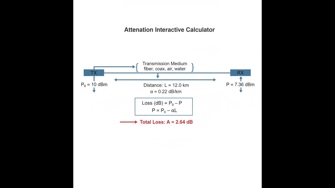
Visual Diagram: Signal Attenuation Through Medium

Attenuation Interactive Calculator

Attenuation Equations

Theory & Practical Applications of Signal Attenuation

Signal attenuation represents the reduction in power or amplitude as electromagnetic waves, acoustic signals, or optical pulses propagate through transmission media. Unlike free-space path loss which follows inverse-square laws, attenuation in guided media exhibits exponential decay governed by material absorption, scattering, and conversion of electromagnetic or acoustic energy into heat. Understanding attenuation mechanisms is fundamental to link budget analysis, determining repeater spacing, and selecting appropriate transmission technologies for specific distance and bandwidth requirements.

Physical Mechanisms of Attenuation

The attenuation coefficient α quantifies the rate of power loss per unit distance and arises from multiple physical processes. In optical fibers, Rayleigh scattering dominates at wavelengths near 1550 nm, where microscopic density fluctuations in the glass matrix scatter photons out of the guided mode. The scattering cross-section scales as λ⁻⁴, explaining why infrared wavelengths experience lower loss than visible light in silica fibers. Material absorption adds wavelength-dependent loss from electronic and molecular resonances — hydroxyl (OH⁻) absorption creates a loss peak near 1383 nm in non-dry fiber, while infrared absorption from Si-O bond stretching increases beyond 1600 nm.

In coaxial cables and waveguides, conductor losses arise from finite conductivity — RF currents concentrate within a skin depth δ = √(2/(ωμσ)), where ω is angular frequency, μ is permeability, and σ is conductivity. Attenuation increases with √f because skin depth decreases, forcing current into smaller cross-sectional areas and increasing resistive losses. Dielectric losses in the insulating material add frequency-dependent attenuation proportional to tan(δ) × f, where tan(δ) is the loss tangent characterizing molecular dipole relaxation.

For underwater acoustic propagation, attenuation combines absorption (converting acoustic energy to heat via viscous friction and molecular relaxation) with scattering from suspended particles, bubbles, and marine life. The Thorp equation models frequency-dependent absorption in seawater: α ≈ 0.11f²/(1 + f²) + 44f²/(4100 + f²) + 2.75×10⁻⁴f² + 0.003 dB/km, where f is in kHz. This cubic frequency dependence severely limits long-range high-frequency sonar — at 100 kHz, absorption alone causes 36 dB/km loss, restricting ranges to hundreds of meters rather than kilometers.

Link Budget Analysis and System Design

Communication system design begins with link budget calculations that account for all gains and losses between transmitter and receiver. The fundamental equation P_RX = P_TX + G_TX - L_path - A_atten + G_RX must exceed the receiver sensitivity S_min with sufficient margin M (typically 3-10 dB) to ensure reliable operation under fading and interference. The attenuation term A_atten = α × L dominates in fiber optic and cable systems, unlike wireless links where free-space path loss L_path = 20log₁₀(4πd/λ) often dominates.

For submarine fiber optic cables spanning oceanic distances, attenuation determines amplifier spacing and system cost. Modern single-mode fibers achieve α ≈ 0.18-0.20 dB/km at 1550 nm wavelength. Over a 6000 km transoceanic route, total attenuation reaches 1080-1200 dB — an astronomical loss requiring erbium-doped fiber amplifiers (EDFAs) every 40-80 km to boost signal power back above the noise floor. Each amplifier adds cost, power consumption, and failure risk, making low-loss fiber development economically critical. Specialty fibers using hollow-core photonic bandgap structures target α below 0.15 dB/km by confining light to air rather than glass, reducing Rayleigh scattering.

In RF coaxial systems, attenuation escalates rapidly with frequency. Standard RG-58 cable exhibits α ≈ 0.2 dB/m at 100 MHz but 0.66 dB/m at 1 GHz — a 3.3× increase for 10× frequency. This forces cellular base station installations to minimize cable runs between antenna and transceiver. Low-loss alternatives like LMR-400 or 7/8" hardline reduce loss to 0.07 dB/m at 1 GHz but cost significantly more and require professional installation. The economic tradeoff balances cable cost against signal loss — a 50-meter run of RG-58 loses 33 dB at 1 GHz (reducing power by 99.95%), necessitating higher transmitter power or better cable despite cost.

Worked Example: Fiber Optic Network Design

Problem: A telecommunications provider is designing a metro fiber optic network connecting a central office to a remote cell tower 47.3 km away. The optical transmitter outputs +3.0 dBm at 1550 nm wavelength into single-mode fiber with attenuation coefficient α = 0.21 dB/km. The receiver requires minimum optical power of -28.0 dBm for 10⁻¹² bit error rate at 10 Gbps data rate. Connector and splice losses total 2.8 dB across the entire link. Determine: (a) Total link attenuation, (b) Received optical power without amplification, (c) Link margin relative to receiver sensitivity, (d) Whether amplification is required, and (e) If amplification is needed, calculate optimal location and output power for a single mid-span EDFA.

Solution:

(a) Total Link Attenuation:
Fiber attenuation: A_fiber = α × L = 0.21 dB/km × 47.3 km = 9.933 dB
Connector/splice losses: A_conn = 2.8 dB
Total attenuation: A_total = 9.933 + 2.8 = 12.733 dB

(b) Received Optical Power:
P_RX = P_TX - A_total
P_RX = +3.0 dBm - 12.733 dB = -9.733 dBm

(c) Link Margin:
Margin = P_RX - S_min = -9.733 dBm - (-28.0 dBm) = +18.267 dB

This substantial positive margin indicates the link operates well above the receiver sensitivity threshold. No amplification is required — the system has 18.3 dB of margin to accommodate aging (fiber attenuation increases ≈0.01 dB/km per decade), additional splices during maintenance, or future upgrades to higher data rates requiring better signal-to-noise ratio.

(d) Amplification Assessment:
Amplification is NOT required. Standard practice demands 3-6 dB minimum margin; this link has 18.3 dB, providing robust operation with room for component degradation over the system's 25-year design life.

(e) Hypothetical Amplifier Design (for learning purposes):
If the distance were extended to 180 km (maintaining α = 0.21 dB/km), fiber loss would reach 37.8 dB plus 2.8 dB connector losses = 40.6 dB total. Received power would be +3.0 - 40.6 = -37.6 dBm, falling 9.6 dB below the -28.0 dBm sensitivity — amplification would then be mandatory.

For a single mid-span amplifier at the 90 km midpoint:
Loss from TX to amplifier: 0.21 × 90 + 1.4 = 20.3 dB
Power into amplifier: +3.0 - 20.3 = -17.3 dBm
Required amplifier output to meet -28.0 dBm at RX with 3 dB margin:
P_amp-out = -25.0 dBm + 20.3 dB = -4.7 dBm
Amplifier gain required: -4.7 - (-17.3) = +12.6 dB

This modest gain requirement suits standard EDFA designs operating well below saturation power, ensuring low noise figure (typically 4-5 dB for small-signal EDFAs) and minimal nonlinear distortion.

Industry Applications and Standards

For more link budget and system design tools, visit our engineering calculator library which includes RF path loss calculators, antenna gain tools, and modulation scheme analyzers.

Telecommunications standards specify maximum attenuation coefficients for different fiber types and applications. ITU-T G.652 (standard single-mode fiber) allows α ≤ 0.40 dB/km at 1310 nm and ≤ 0.30 dB/km at 1550 nm for deployed cable — manufacturers typically achieve 0.33 dB/km and 0.19 dB/km respectively, providing margin against specification. ITU-T G.657 bend-insensitive fiber trades slightly higher straight-section loss (α ≈ 0.22 dB/km at 1550 nm) for dramatically reduced macro-bend loss, enabling tighter routing radii in building installations where space constraints force 15-30 mm bend radii that would cause catastrophic loss in standard fiber.

Coaxial cable manufacturers publish attenuation versus frequency curves allowing system designers to select appropriate cable types. Cellular distributed antenna systems (DAS) in large buildings must balance cable loss against installation cost — longer runs to reach all coverage zones increase attenuation, requiring more RF power at the source or additional amplifiers. A 150-meter LMR-400 run at 2.1 GHz (UMTS Band I) loses 10.5 dB, equivalent to reducing effective radiated power by 91.1%. If the base station outputs +43 dBm (20 watts) into this cable, only +32.5 dBm (1.78 watts) reaches the antenna. For dense urban coverage requiring multiple antennas, fiber-fed remote radio heads (RRHs) eliminate coaxial loss by locating RF electronics at antenna locations, transmitting digitized baseband over low-loss fiber.

Underwater acoustic communication systems face extreme attenuation constraints that fundamentally limit data rates and ranges. At 10 kHz center frequency suitable for kilometer-scale ranges, absorption contributes ≈0.9 dB/km, while geometric spreading adds 20log₁₀(r) loss. A 5 km link experiences 4.5 dB absorption plus 20log₁₀(5000) ≈ 74 dB spreading loss = 78.5 dB total, forcing transmit powers of 180-190 dB re 1 μPa to achieve 100-110 dB re 1 μPa receive levels above ambient noise. Raising frequency to 50 kHz for higher data rates increases absorption to 22.5 dB/km — the 5 km path now loses 112.5 + 74 = 186.5 dB, rendering long-range communication impractical without relay nodes spaced at 1-2 km intervals.

Temperature and Environmental Effects

Attenuation coefficients exhibit temperature dependence that impacts system performance over environmental ranges. Optical fiber attenuation increases ≈0.0001 dB/km per °C due to changes in glass density affecting Rayleigh scattering. Over -40°C to +70°C operating range (110°C span), a 50 km fiber link experiences 0.55 dB additional loss at temperature extremes — negligible for well-margined systems but potentially significant for long submarine cables operating near receiver sensitivity limits.

Coaxial cable attenuation varies with temperature through thermal expansion affecting conductor spacing and resistivity changes. LMR-400 attenuation increases approximately 0.15% per °C above 20°C reference — at 70°C, loss increases 7.5% over nominal. For a 100-meter run with 7.0 dB loss at 20°C, high temperature raises loss to 7.53 dB, consuming 0.53 dB of link margin. Military and aerospace systems account for these variations in worst-case link budgets.

Seawater attenuation depends strongly on temperature, salinity, and pH affecting molecular relaxation rates. Acoustic absorption increases ≈3% per °C in the 0-30°C range relevant to ocean environments. Seasonal thermocline variations alter sound speed profiles, creating convergence zones and shadow zones that modulate propagation loss by 10-20 dB beyond simple attenuation predictions — requiring adaptive communication protocols that adjust modulation, coding, and transmit power based on measured channel conditions.

Frequently Asked Questions