Control Chart Xbar R Interactive Calculator

The X̄-R (X-bar R) control chart is a statistical process control tool used to monitor the mean and variability of a manufacturing process over time. By plotting sample means (X̄) and ranges (R) against calculated control limits, quality engineers can detect process shifts, trends, or out-of-control conditions before they result in defective products. This calculator generates Upper Control Limits (UCL), Lower Control Limits (LCL), and centerlines for both X̄ and R charts based on your sample data, enabling real-time process monitoring and continuous improvement initiatives.

📐 Browse all free engineering calculators

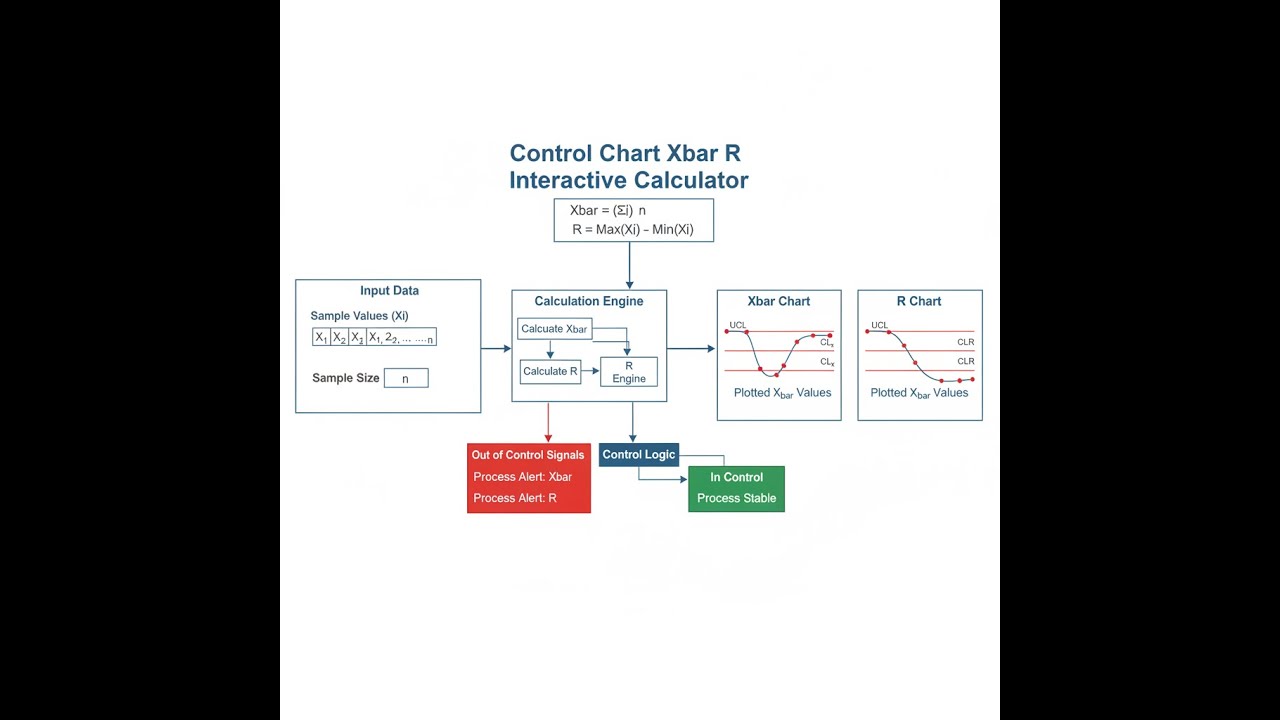
Visual Diagram

Control Chart X̄-R Calculator

Control Chart Equations

Theory & Engineering Applications

Statistical Foundation of X̄-R Control Charts

The X̄-R control chart system represents one of the most widely implemented statistical process control (SPC) tools in manufacturing, developed by Walter Shewhart at Bell Laboratories in the 1920s. Unlike simple specification checking, which only identifies defects after production, control charts enable real-time detection of process shifts and trends, allowing operators to intervene before defective parts are produced. The dual-chart approach monitors both process location (X̄ chart) and process dispersion (R chart) simultaneously, providing complete visibility into process behavior.

The theoretical basis relies on the Central Limit Theorem, which states that the distribution of sample means approaches normality regardless of the underlying population distribution, provided the sample size is adequate (typically n ≥ 4). This normality assumption justifies the use of ±3σ limits, which capture approximately 99.73% of variation when the process operates in statistical control. The range (R) provides a computationally simple estimator of process variability, though it becomes less efficient than standard deviation for sample sizes exceeding 10-12 units.

Control Chart Constants and Their Derivation

The constants A₂, D₃, D₄, and d₂ are derived from the sampling distribution of the range statistic. The relationship d₂ = E(R)/σ represents the expected value of the range divided by the population standard deviation, allowing us to estimate σ from observed ranges. For a sample size of n=5, d₂ equals 2.326, meaning the average range is approximately 2.326 times the standard deviation. The A₂ constant combines the 3σ multiplier with the d₂ relationship and the standard error of the mean (σ/√n), resulting in A₂ = 3/(d₂√n) = 0.577 for n=5.

A critical limitation often overlooked in textbook treatments: these constants assume rational subgrouping, where measurements within a subgroup represent instantaneous or near-instantaneous production under homogeneous conditions. Violating this assumption by including multiple production runs, operators, or machine setups within a single subgroup inflates the within-subgroup variation, leading to wider control limits that mask assignable causes. The between-subgroup variation should capture process changes over time, while within-subgroup variation represents inherent process noise.

Phase I vs Phase II Control Charting

Manufacturing engineers must distinguish between Phase I (chart development) and Phase II (ongoing monitoring). During Phase I, historical data establishes initial control limits, but these limits are tentative. Any out-of-control points indicate assignable causes that must be investigated and, if confirmed, removed from the dataset before recalculating limits. This iterative process continues until the data demonstrates statistical control. Only then do the limits become reliable standards for Phase II monitoring. Many quality failures occur because organizations skip Phase I entirely, applying arbitrary limits without statistical validation.

Phase II monitoring introduces additional run rules beyond simple limit violations. The Western Electric Rules detect non-random patterns: 2 out of 3 consecutive points beyond 2σ from centerline, 4 out of 5 consecutive points beyond 1σ, 8 consecutive points on one side of centerline, or 15 consecutive points within 1σ (indicating over-adjustment). These rules increase sensitivity to small process shifts at the cost of slightly higher false alarm rates. Engineers must balance sensitivity against the operational disruption caused by unnecessary investigations.

Process Capability and Control Relationship

A fundamental misconception equates control with capability. A process in statistical control (stable, predictable variation) may still produce unacceptable parts if the natural process spread exceeds specification limits. Process capability indices quantify this relationship. C_p = (USL - LSL)/(6σ̂) measures potential capability assuming perfect centering, while C_pk accounts for actual process centering by taking the minimum of upper and lower capability indices. Industry standards typically require C_pk ≥ 1.33, ensuring at least 4σ distance between process mean and nearest specification limit, corresponding to approximately 64 defects per million opportunities.

The range-based estimator σ̂ = R̄/d₂ provides only short-term variability, excluding between-subgroup variation. For true long-term capability, engineers should use overall standard deviation calculated from individual measurements. This distinction becomes critical in high-volume automotive and aerospace applications where even minor underestimation of variability leads to capability predictions that fail to materialize in production. The automotive industry's PPAP (Production Part Approval Process) explicitly requires both short-term (machine capability) and long-term (process performance) indices.

Practical Implementation Challenges

Real-world implementation encounters several technical challenges. Measurement system analysis (MSA) must precede control charting because measurement variability inflates apparent process variation. If gage R&R exceeds 30% of tolerance or process variation, the measurement system itself requires improvement. Autocorrelation in continuous processes violates the independence assumption underlying control charts, requiring either time-series models or increased sampling intervals to eliminate serial correlation. Multi-stream processes (parallel machines producing identical parts) require individual charts for each stream plus rational between-stream comparison methods.

For additional statistical process control resources and manufacturing calculators, visit the engineering calculator library.

Worked Example: Pharmaceutical Tablet Production

A pharmaceutical manufacturer produces 500mg acetaminophen tablets with specification limits of 485-515mg. Quality control collects samples of n=5 tablets every 30 minutes during an 8-hour shift, measuring individual tablet weights with a calibrated analytical balance (resolution 0.1mg). Over 20 sampling intervals, the following data is recorded:

Sample Means (X̄, in mg): 499.2, 501.3, 498.7, 502.1, 500.5, 499.8, 501.6, 500.2, 498.9, 501.4, 499.5, 500.8, 502.3, 499.1, 500.6, 501.9, 499.3, 500.4, 501.1, 499.7

Sample Ranges (R, in mg): 3.2, 4.1, 3.8, 4.5, 3.6, 3.9, 4.2, 3.5, 3.7, 4.3, 3.4, 4.0, 4.6, 3.3, 3.8, 4.4, 3.6, 3.9, 4.1, 3.7

Step 1: Calculate Grand Mean (X̄̄)

Sum of sample means = 499.2 + 501.3 + ... + 499.7 = 10,008.3 mg

X̄̄ = 10,008.3 / 20 = 500.415 mg

Step 2: Calculate Average Range (R̄)

Sum of ranges = 3.2 + 4.1 + ... + 3.7 = 78.6 mg

R̄ = 78.6 / 20 = 3.93 mg

Step 3: Determine Control Chart Constants for n=5

From standard tables: A₂ = 0.577, D₃ = 0, D₄ = 2.114, d₂ = 2.326

Step 4: Calculate X̄ Chart Limits

UCL_X̄ = X̄̄ + A₂R̄ = 500.415 + (0.577)(3.93) = 500.415 + 2.268 = 502.683 mg

CL_X̄ = 500.415 mg

LCL_X̄ = X̄̄ - A₂R̄ = 500.415 - 2.268 = 498.147 mg

Step 5: Calculate R Chart Limits

UCL_R = D₄R̄ = (2.114)(3.93) = 8.308 mg

CL_R = 3.93 mg

LCL_R = D₃R̄ = (0)(3.93) = 0 mg (no lower limit for n≤6)

Step 6: Assess Process Capability

Estimate standard deviation: σ̂ = R̄/d₂ = 3.93/2.326 = 1.690 mg

C_p = (USL - LSL)/(6σ̂) = (515 - 485)/(6 × 1.690) = 30/10.140 = 2.96

Upper capability: (515 - 500.415)/(3 × 1.690) = 14.585/5.070 = 2.88

Lower capability: (500.415 - 485)/(3 × 1.690) = 15.415/5.070 = 3.04

C_pk = min(2.88, 3.04) = 2.88

Interpretation: All sample means fall within control limits (498.147 to 502.683 mg), and all ranges remain below the upper control limit of 8.308 mg, indicating the process operates in statistical control. The C_pk value of 2.88 significantly exceeds the pharmaceutical industry standard of 1.33, indicating excellent process capability with minimal risk of producing out-of-specification tablets. The process mean of 500.415 mg sits nearly perfectly centered between specification limits, with approximately 9.6σ distance to the nearest specification boundary, corresponding to defect rates below 1 part per billion. This exceptional capability allows the manufacturer to confidently maintain production without excessive sampling or risk of batch rejection.

Practical Applications

Frequently Asked Questions