Wave Speed Interactive Calculator

The Wave Speed Interactive Calculator computes the propagation velocity of mechanical and electromagnetic waves using the fundamental relationship between frequency, wavelength, and wave speed. This tool serves physicists, RF engineers, acousticians, and optical designers who need to analyze wave behavior across media—from seismic waves traveling through Earth's crust at 8 km/s to fiber optic signals propagating at 2×10⁸ m/s through glass. Understanding wave speed is critical for designing communication systems, ultrasonic testing equipment, and predicting wave interference patterns in complex environments.

📐 Browse all free engineering calculators

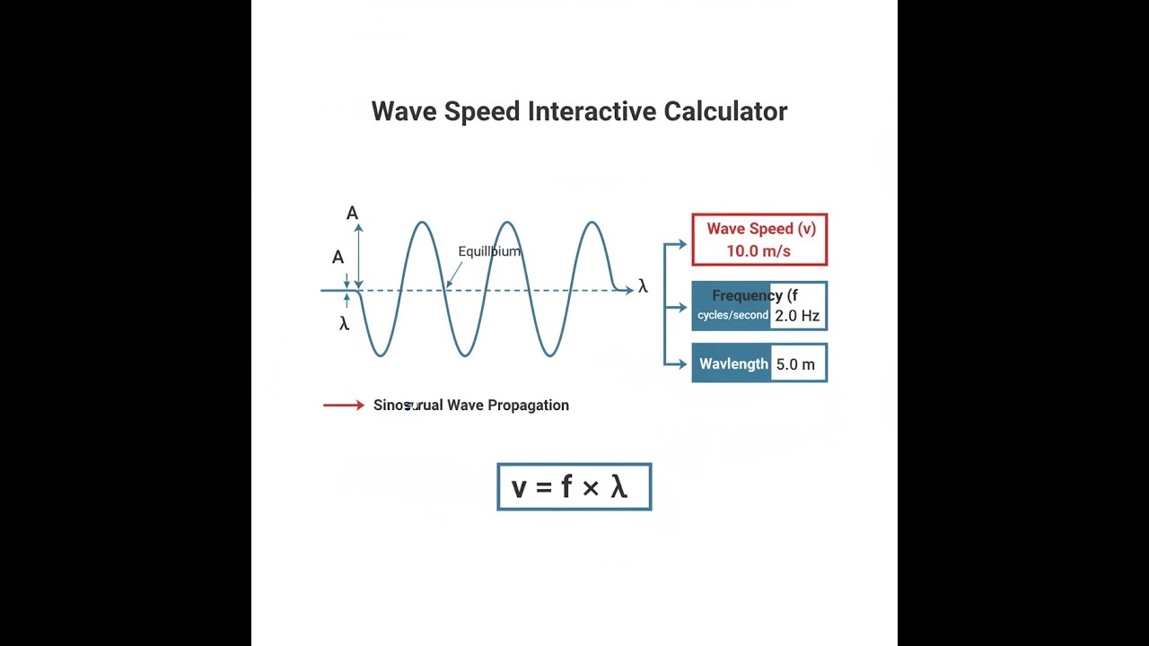
Wave Propagation Diagram

Interactive Wave Speed Calculator

Wave Speed Equations

Theory & Practical Applications

Fundamental Wave Physics and Dispersion Relations

The wave speed equation v = fλ represents one of the most profound relationships in physics, unifying oscillatory phenomena across twelve orders of magnitude in frequency—from seismic waves at 0.01 Hz to gamma rays at 10²⁰ Hz. This equation emerges directly from the definition of wavelength as the spatial period of a wave: if a wave oscillates f times per second and each oscillation propagates a distance λ, the wave must advance a total distance fλ each second. What makes this relationship non-trivial is that wave speed itself depends on the medium's physical properties, creating frequency-dependent propagation in dispersive media—a phenomenon that limits fiber optic bandwidth and causes musical instruments to sound inharmonic at high amplitudes.

In non-dispersive media like vacuum for electromagnetic waves or ideal strings under small displacement, all frequency components travel at identical speed, preserving pulse shapes over arbitrary distances. This property underlies GPS timing precision: satellite signals at 1.57542 GHz maintain coherence across 20,200 km because vacuum dispersion is exactly zero. Conversely, dispersive media like optical fiber exhibit frequency-dependent refractive index n(f), causing different spectral components of a signal pulse to arrive at different times—a phenomenon called group velocity dispersion that telecommunications engineers combat using chirped fiber Bragg gratings and dispersion-compensating fiber segments to maintain signal integrity over transoceanic distances exceeding 10,000 km.

Medium-Specific Propagation Mechanisms

Sound waves in gases propagate through sequential compression and rarefaction of molecules, with speed determined by the gas's compressibility and density. The temperature dependence v ∝ √T arises because molecular kinetic energy increases with temperature, accelerating the momentum transfer between colliding molecules. This creates a 0.6 m/s increase per °C in air—critical for outdoor sound system alignment where temperature gradients between stage and audience can shift wavefront arrival by several milliseconds, causing destructive interference in the 2-4 kHz intelligibility band. Professional audio engineers measure on-site temperature profiles and apply time-alignment delays to compensate for the spatial variation in sound speed, maintaining coherent summation of arrayed loudspeaker elements.

Electromagnetic waves in dielectric materials slow according to v = c/n, where refractive index n quantifies the material's polarizability—how readily its electron clouds distort in response to the oscillating electric field. This distortion creates secondary wavelets that interfere with the incident wave, producing a net phase delay equivalent to reduced propagation speed. The frequency dependence of n causes chromatic aberration in lenses: blue light (n = 1.532 for BK7 glass at 486 nm) refracts more strongly than red light (n = 1.514 at 656 nm), requiring achromatic doublets combining crown and flint glass elements with opposing dispersion to bring multiple wavelengths to a common focus. Modern fiber optics operate in the 1550 nm telecommunications window where silica glass exhibits both minimum absorption (0.2 dB/km) and near-zero dispersion slope, allowing 100 Gb/s signals to propagate 80 km without regeneration.

Mechanical Waves and Material Properties

Transverse waves on strings exhibit speed v = √(T/μ) because wave propagation requires both restoring force (tension T) and inertia (linear density μ). Higher tension increases the restoring force gradient, accelerating disturbances, while higher mass density increases inertia, slowing propagation. Guitar string manufacturers exploit this relationship: a high-E string (steel, μ = 0.00038 kg/m) at 72 N tension produces 329.6 Hz at 0.648 m length, while the low-E string (wound phosphor bronze, μ = 0.0038 kg/m) requires only 68 N for 82.4 Hz at the same length. The ten-fold density difference compensates for the minimal tension variation, demonstrating how material selection enables precise frequency control without structural loading concerns.

Seismic waves reveal Earth's internal structure through velocity variations with depth. Primary (P) waves—longitudinal compression waves—travel at 5-7 km/s through continental crust, accelerating to 13.7 km/s in the iron-nickel inner core as incompressibility increases. Secondary (S) waves—transverse shear waves—propagate at roughly 60% of P-wave speed in the same medium, but cannot traverse the liquid outer core where shear modulus vanishes. The 103-second delay between P and S wave arrival at a seismometer 1000 km from an epicenter reveals both wave speeds and epicentral distance through the equation Δt = d(1/v_S - 1/v_P). Seismologists use these differential travel times across global station networks to tomographically image mantle convection cells and subducting slabs with 50 km spatial resolution.

Worked Multi-Part Engineering Example: Fiber Optic Link Budget

Problem: A telecommunications provider designs a 65 km fiber optic link operating at 1550 nm wavelength. The single-mode fiber has refractive index n = 1.4682 at this wavelength. A 10 Gb/s NRZ signal requires pulse duration of at least 100 ps to avoid intersymbol interference. Calculate: (a) propagation speed in the fiber, (b) signal propagation delay, (c) maximum frequency component in the 10 Gb/s signal assuming 5th harmonic bandwidth, (d) wavelength of this frequency component in the fiber, and (e) verify that chromatic dispersion with D = 17 ps/(nm·km) doesn't violate the 100 ps pulse width requirement.

Solution:

Part (a): Speed in fiber using v = c/n
v = (2.998 × 10⁸ m/s) / 1.4682
v = 2.0417 × 10⁸ m/s
This represents a 31.9% reduction from vacuum speed—significant for synchronization systems.

Part (b): Propagation delay t = distance / speed
t = 65,000 m / (2.0417 × 10⁸ m/s)
t = 3.183 × 10^-4 s = 318.3 μs
This one-way latency must be doubled for acknowledgment-based protocols.

Part (c): Fifth harmonic of 10 Gb/s signal
Fundamental frequency = 10 × 10⁹ Hz / 2 = 5 GHz (NRZ bandwidth)
f₅ = 5 × 5 GHz = 25 GHz
Practical systems filter beyond 3rd harmonic, but 5th harmonic calculation demonstrates worst-case dispersion.

Part (d): Wavelength in fiber at 25 GHz optical frequency
The carrier wavelength is 1550 nm. Converting to frequency:
f_carrier = c / λ_vacuum = (2.998 × 10⁸) / (1550 × 10^-9) = 1.9342 × 10¹⁴ Hz
The 25 GHz modulation appears as sidebands at f_carrier ± 25 GHz
Upper sideband: f_upper = 1.9342 × 10¹⁴ + 25 × 10⁹ = 1.93420025 × 10¹⁴ Hz
Wavelength in fiber: λ_fiber = v / f = (2.0417 × 10⁸) / (25 × 10⁹) = 0.00817 m = 8.17 mm
This represents the spatial period of the modulation envelope traveling through the fiber.

Part (e): Chromatic dispersion penalty
Dispersion coefficient D = 17 ps/(nm·km) specifies pulse spreading per nm of source bandwidth per km of fiber.
For a 10 Gb/s signal, spectral width from modulation is approximately:
Δλ = (λ² / c) × Δf = (1550 × 10^-9)² / (2.998 × 10⁸) × (10 × 10⁹) = 0.080 nm
Pulse spreading: σ_dispersion = D × Δλ × L = 17 × 0.080 × 65 = 88.4 ps
Since 88.4 ps is less than the 100 ps pulse slot, the link meets timing requirements with 11.6 ps margin. However, this assumes ideal conditions—real systems would use dispersion compensation beyond 50 km to maintain margin for temperature variations and aging.

Applications Across Engineering Disciplines

In ultrasonic nondestructive testing, longitudinal waves at 5 MHz propagate through steel at 5,960 m/s, yielding wavelength λ = 1.19 mm. Defect detection resolution scales with wavelength—flaws smaller than λ/2 ≈ 0.6 mm scatter minimally and remain undetectable. Inspectors must select frequency based on the minimum flaw size of concern: 10 MHz for aerospace turbine blade inspection (0.3 mm cracks), versus 1 MHz for large forging inspection where 6 mm voids are the failure threshold. The wave speed in the test material determines required transducer standoff distance and time-of-flight calibration for thickness measurement with 0.01 mm precision.

Radar systems measure target range through time-of-flight: r = ct/(2n), where the factor of 2 accounts for round-trip propagation and n corrects for atmospheric refraction (n ≈ 1.0003 at sea level, increasing with humidity). A 94 GHz millimeter-wave radar measuring drone altitude at 100 m altitude experiences 667 ns round-trip delay. At this frequency, λ = 3.19 mm in air, requiring phase-coherent processing to resolve targets separated by less than 10 cm through Doppler frequency shifts of ±3 kHz per m/s of radial velocity. Weather radar operates at longer wavelengths (10 cm at S-band) specifically because Rayleigh scattering from raindrops scales as λ^-4—shorter wavelengths would saturate from excessive atmospheric return.

Advanced Topics and Edge Cases

Wave packets in dispersive media exhibit distinct phase and group velocities. Phase velocity v_p = ω/k describes individual wavefront propagation, while group velocity v_g = dω/dk governs energy transport and signal propagation. In anomalous dispersion regions of optical fiber near 1300 nm, v_g can exceed v_p, and in metamaterials with negative refractive index, phase and group velocities oppose each other directionally. Optical solitons exploit the precise balance between group velocity dispersion and self-phase modulation through the Kerr nonlinearity to propagate undistorted over thousands of kilometers—enabling transoceanic links without electronic regeneration by maintaining the temporal and spectral shape through a fortuitous cancellation of normally destructive effects.

Near-field effects complicate the simple v = fλ relationship when source dimensions become comparable to wavelength. A 40 kHz ultrasonic transducer with 10 mm diameter generates a near-field zone extending N = D²f/(4v) = (0.01)² × 40000 / (4 × 343) = 0.29 m, within which the wavefront exhibits complex interference patterns unsuitable for distance measurement. Only beyond this transition distance does the far-field inverse-square intensity law apply—critical for calibrating proximity sensors and medical ultrasound imaging systems where resolution and intensity calculations assume spherical wave propagation.

For engineers working across domains, explore our complete library of free engineering calculators covering mechanics, thermodynamics, electromagnetics, and fluid dynamics—each designed with the same level of technical depth and practical applicability.

Frequently Asked Questions