Mirror Equation Interactive Calculator

The mirror equation calculator determines the relationship between object distance, image distance, and focal length for curved mirrors. Essential for optical system design, telescopes, solar concentrators, and machine vision applications, this tool enables engineers to predict image formation characteristics and optimize mirror geometries for specific magnification and focusing requirements.

📐 Browse all free engineering calculators

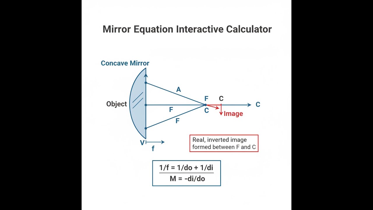
Mirror Geometry Diagram

Interactive Mirror Equation Calculator

Mirror Equation Formulas

Theory & Practical Applications of Mirror Equations

The mirror equation represents one of the fundamental relationships in geometric optics, governing image formation by spherical mirrors through the paraxial approximation. Unlike the more general ray-tracing approach, the mirror equation provides direct analytical prediction of image characteristics based solely on object position and mirror curvature, enabling rapid optical system optimization without iterative numerical methods.

Derivation and Physical Basis

The mirror equation emerges from Fermat's principle applied to spherical reflecting surfaces. For a concave mirror with radius of curvature R, the focal point lies at f = R/2, where parallel rays converge after reflection. The relationship 1/f = 1/d_o + 1/d_i follows directly from similar triangles formed by incident and reflected rays intersecting the principal axis. This derivation assumes small angle approximations (paraxial rays), limiting accuracy for rays far from the optical axis or mirrors with large apertures relative to their radius of curvature.

A critical non-obvious limitation emerges when objects approach the focal point. As d_o → f, the image distance d_i approaches infinity — the image forms at an increasingly distant position. Mathematically, when d_o = f exactly, the equation yields 1/d_i = 0, representing image formation at infinity where rays emerge parallel. This regime defines the collimation condition exploited in astronomical telescopes and laser beam expanders. For practical mirrors with finite aperture, aberrations and diffraction effects become dominant at this boundary, and the idealized thin-mirror equation breaks down.

Sign Convention and Physical Interpretation

The negative sign in the magnification equation m = -d_i/d_o embeds fundamental geometric information about ray paths. For concave mirrors forming real images (d_o > f), both d_o and d_i are positive, yielding negative magnification — indicating image inversion relative to the object. When d_o < f, the equation predicts negative d_i, signifying a virtual image formed by backward extension of reflected rays. This virtual image appears upright (positive magnification) and enlarged, as exploited in magnifying makeup mirrors and dental examination mirrors.

The sign convention for focal length distinguishes converging mirrors (f < 0, concave) from diverging mirrors (f > 0, convex). Convex mirrors always produce virtual, upright, reduced images regardless of object position, making them ideal for wide-field surveillance and automotive side mirrors where field of view outweighs magnification. The mirror equation applies equally to both types, though convex mirrors yield only negative image distances in all physically realizable configurations.

Spherical Aberration and Validity Limits

The mirror equation's paraxial approximation fails for rays striking the mirror far from its center. Spherical aberration causes peripheral rays to focus at different points than central rays, degrading image sharpness. For a spherical mirror of radius R and aperture diameter D, the longitudinal spherical aberration scales as Δz ≈ D⁴/(128R³f), showing quartic dependence on aperture. This explains why large astronomical mirrors use parabolic profiles rather than spherical surfaces — paraboloids eliminate spherical aberration for on-axis objects at the cost of increased fabrication complexity.

Practical optical designers must balance mirror aperture against acceptable aberration levels. Solar concentrators for thermal power generation operate with f/D ratios (focal length to diameter) typically between 0.6 and 1.2, accepting spherical aberration in exchange for manufacturing economy. High-precision telescope primary mirrors require f/D > 3 to maintain diffraction-limited performance using spherical surfaces, or employ aspherical figures for faster systems.

Industrial Applications Across Sectors

Satellite ground station antennas exploit the mirror equation's electromagnetic equivalence — radiofrequency waves obey identical reflection laws as visible light. A parabolic dish antenna with focal length f = 2.4 m and diameter D = 3.5 m operates at f/D = 0.686, focusing downlink signals from geostationary satellites 35,786 km distant. The feed horn must be positioned exactly at the focal point to maximize gain, and thermal expansion of the support structure requires active focus correction to maintain alignment across temperature ranges from -30°C to +50°C.

Solar furnaces use large concave mirrors to concentrate sunlight for materials processing at temperatures exceeding 3000°C. The Odeillo solar furnace in France employs a 54-meter-diameter parabolic mirror (f = 18 m) achieving concentration ratios of 10,000:1. At such extreme concentration, ray-tracing analysis becomes essential because the large aperture violates paraxial assumptions. The mirror equation provides initial design values, but final optimization requires Monte Carlo ray tracing accounting for solar disk angular extent (0.53°), mirror surface errors (typically 2-5 mrad RMS slope error), and atmospheric turbulence effects.

Laser cavity design for industrial cutting systems critically depends on mirror equation calculations. A typical 5 kW fiber laser cutting head uses an aspheric focusing mirror with effective focal length f = 127 mm to produce a focal spot diameter of 180 μm at the workpiece. The mirror must maintain focus across a working range of ±2 mm while the motion system moves the head at up to 200 m/min. Thermal lensing from absorbed laser power (even 0.1% absorption equals 5 W heating) shifts the focal point according to Δf ≈ αP/(κA), where α is thermal expansion coefficient, κ is thermal conductivity, P is absorbed power, and A is mirror area. Active cooling systems with temperature control to ±0.5°C are required to maintain focus within the ±50 μm Rayleigh range.

Multi-Mirror Systems and Optical Path Analysis

Cassegrain telescope configurations use both concave and convex mirrors in series, requiring careful application of the mirror equation to each surface sequentially. The primary mirror (f₁ = -800 mm) forms an intermediate real image, which serves as a virtual object (negative object distance) for the convex secondary mirror (f₂ = +200 mm). The effective focal length of the combined system becomes f_eff = f₁f₂/(f₁ + f₂ - d), where d is the mirror separation. For d = 720 mm, this yields f_eff = -1600 mm, doubling the focal length while maintaining compact physical length — critical for space-based telescopes with launch vehicle diameter constraints.

Beam steering systems in laser materials processing use rapidly tilting mirrors (galvanometric scanners) that must maintain focus across the entire working field. A flat scanning mirror at distance L from a focusing mirror introduces position-dependent defocus according to δ = L²/(2f) for scan angle θ, requiring dynamic focus correction or F-theta lens systems that linearize the scan field. The mirror equation guides initial lens selection, but final optimization requires numerical ray tracing through the complete optical system including workpiece tilt effects.

Worked Example: Astronomical Telescope Primary Mirror Design

An amateur astronomer designs a Newtonian telescope with a 250 mm diameter primary mirror intended for planetary imaging. The design requires f/6 focal ratio for manageable tube length while maintaining acceptable optical quality. Calculate the required focal length, determine image characteristics for Mars (disk diameter 17.9 arcseconds at opposition, distance 78 million km), and evaluate whether spherical aberration will limit performance.

Step 1: Calculate focal length from f/D ratio

Given f/D = 6 and D = 250 mm:

f = 6 × 250 mm = 1500 mm = 1.5 m

For a spherical mirror, radius of curvature R = 2f = 3000 mm = 3.0 m

Step 2: Determine Mars image size using magnification equation

Mars subtends angle θ = 17.9 arcseconds = 17.9 × (π/648000) radians = 8.677 × 10⁻⁵ rad

At Mars distance d_o = 78 × 10⁹ m (treating as object distance), actual diameter:

h_o = θ × d_o = 8.677 × 10⁻⁵ × 78 × 10⁹ = 6.768 × 10⁶ m = 6768 km

Since Mars is effectively at infinity (d_o >> f), rays arrive essentially parallel and focus at the focal point. Image forms at d_i = f = 1500 mm. For objects at infinity, image height:

h_i = f × tan(θ) ≈ f × θ (for small angles) = 1500 mm × 8.677 × 10⁻⁵ rad = 0.130 mm = 130 μm

Step 3: Evaluate spherical aberration limit

Longitudinal spherical aberration for spherical mirror:

Δz = D⁴/(128R³) = (250)⁴/(128 × (3000)³) = 390,625,000,000/(128 × 27,000,000,000) = 0.113 mm

Rayleigh criterion for diffraction-limited imaging requires wavefront error < λ/4. At λ = 550 nm (green light), longitudinal error converts to wavefront error by:

Wavefront error ≈ Δz/(16(f/D)²) = 0.113 mm/(16 × 36) = 0.000196 mm = 196 nm

This equals 196 nm / 550 nm = 0.36 wavelengths, which exceeds λ/4 = 137.5 nm

Step 4: Resolution analysis and practical assessment

Diffraction-limited resolution (Rayleigh criterion): θ_min = 1.22λ/D = 1.22 × 550 × 10⁻⁹ m / 0.25 m = 2.684 × 10⁻⁶ rad = 0.55 arcseconds

Mars disk (17.9 arcseconds) is 32.5 times larger than resolution limit, so disk will be well-resolved. However, spherical aberration will slightly soften fine surface details. For planetary imaging, this f/6 spherical mirror performs acceptably but not optimally. An f/8 design (f = 2000 mm) would reduce spherical aberration to ~48 nm wavefront error, achieving diffraction-limited performance at the cost of longer tube length.

Step 5: Eyepiece selection for viewing

Using a 10 mm focal length eyepiece, total magnification: M = f_mirror/f_eyepiece = 1500/10 = 150×

Mars will appear as a disk of angular size: 17.9" × 150 = 2685" = 44.75 arcminutes = 0.746° as seen by the observer's eye

Exit pupil diameter: D_ep = D/M = 250/150 = 1.67 mm (appropriate for dark-adapted eye with 7 mm pupil)

This worked example demonstrates how the mirror equation integrates with aberration theory, diffraction limits, and practical system design to guide optical engineering decisions. The spherical mirror proves adequate for this application despite exceeding ideal wavefront error limits, because atmospheric seeing typically limits ground-based telescopes to ~1 arcsecond resolution anyway — making ultra-precise optics unnecessary for amateur planetary observation.

Thermal Effects in Precision Mirror Systems

High-power laser applications introduce thermal distortions that effectively change mirror focal length dynamically. A copper mirror absorbing 50 W from a 10 kW CO₂ laser beam (0.5% absorptivity) experiences center-to-edge temperature gradients producing thermal lensing. The focal length shift follows ΔF = κF²/(αP), where κ = 400 W/(m·K) for copper and α = 17 × 10⁻⁶ K⁻¹. For F = 200 mm and P = 50 W, this yields ΔF ≈ 9.4 mm — a significant fraction of the focal length requiring active compensation or water cooling to maintain beam focus.

Aerospace applications confront additional challenges from pressure differentials across mirror surfaces. Satellite telescope mirrors transitioning from ground testing (1 atm) to orbital vacuum experience differential deflection of optical surfaces unless specifically designed with ventilation paths. A 300 mm diameter mirror 25 mm thick deflects by δ = (P × D⁴)/(64Et³) where E is elastic modulus and t is thickness. For Zerodur glass-ceramic (E = 91 GPa), this produces ~2 μm of center deflection under 1 atm pressure differential — enough to completely defocus an f/6 system. Vacuum testing during integration validates that mirror mounts properly release these loads without degrading optical performance.

For readers designing optical systems beyond simple spherical mirrors, the principles established by the mirror equation extend to aspheric surfaces, gradient-index optics, and adaptive systems through modified ray-tracing algorithms. Visit the engineering calculator library for additional tools covering lens systems, fiber optics, and diffractive optics calculations that complement mirror-based designs.

Frequently Asked Questions